concept_5

ECON 0150 | Economic Data Analysis

The economist’s data analysis pipeline.

Part 5.4 | Causation, Controls, and Model Selection

Today’s Class

Causation, controls, and model selection

Why controls matter: causation vs. correlation
How to compare models: R² and the F-test
How to choose a model: the model selection framework

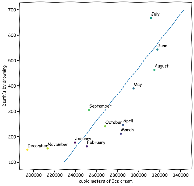
Ice Cream Sales and Drowning Deaths

Monthly data from 12 months.

As ice cream sales go up, so do drowning deaths (\(\hat\beta_1\) = 3.4, p < 0.001)!

Q. So ice cream causes drowning?

Three Possible Explanations

Correlation cannot tell us which explanation is right.

Direct Causation: Ice Cream → Swimming → Drowning
Eating ice cream makes people want to swim?

Reverse Causation: Drowning → Ice Cream Sales
News of drownings drives sympathy ice cream consumption?

Confounding: Something else causes both

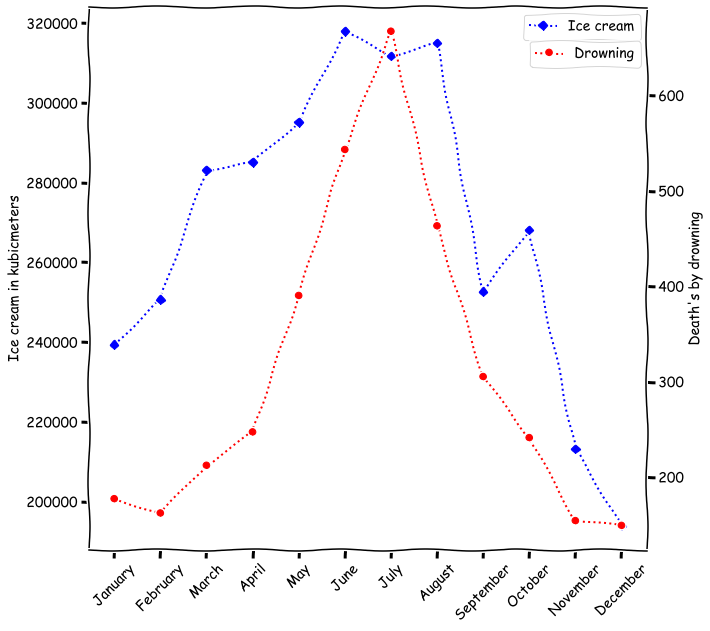
Let’s Look at the Timing

Both variables follow a seasonal pattern.

Both ice cream sales and drowning deaths peak in summer months

The True Relationship

Season is the confounding variable driving both.

The relationship between ice cream and drowning is spurious.

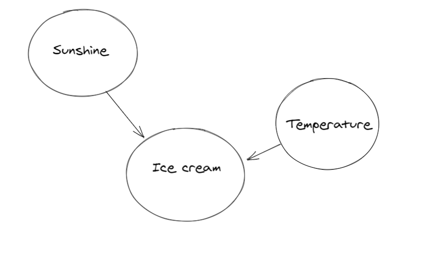
The Fix: Control Variables

Adding the confounder to the model removes the spurious relationship.

Simple model (spurious relationship):

\[\text{Drownings} = \beta_0 + \beta_1 \cdot \text{IceCream} + \varepsilon\]

\(\beta_1 > 0\), highly significant

Controlled model (add the confounder):

\[\text{Drownings} = \beta_0 + \beta_1 \cdot \text{IceCream} + \beta_2 \cdot \text{Temperature} + \varepsilon\]

\(\beta_1\) becomes insignificant, \(\beta_2\) captures the real effect

This Is What The Homework Has Been Doing :)

The BRFSS homework arc is a causation story.

	Model	Control
HW 4.1	BMI ~ unemployment_rate	Nothing
HW 5.1	BMI ~ unemployment_rate + Female	Gender
HW 5.2	BMI ~ unemployment_rate × Female	Gender × effect
HW 5.3	BMI ~ unemployment_rate + Female + AGE + College + Married	Multiple

Each control removes a confounder from the unemployment-BMI relationship.

Controls Don’t Guarantee Causation

Three problems remain, even after adding controls.

1. Omitted variable bias

There might be a confounder we didn’t think of (diet, exercise, genetics…)

2. Reverse causality

Maybe poor health causes unemployment, not the other way around

3. Measurement error

BMI in BRFSS is self-reported, so systematic misreporting could bias results

Controls help, but they can’t prove causation on their own.

Model Comparison

How do we know if adding controls improves the model?

We need tools to compare models:

R²: How much variation does the model explain?
F-test: Is the improvement statistically significant?

R²: Proportion of Variation Explained

How much of the variation does our model capture?

\[R^2 = 1 - \frac{SSE}{SST}\]

\(SST\): total variation (SSE of the mean-only model)
\(SSE\): leftover variation after fitting the model

\(R^2\) measures how much of the variability in the data is captured by the model.

\(R^2 = 0\): model does no better than the mean
\(R^2 = 1\): model predicts perfectly

Q. Is a higher \(R^2\) always better?

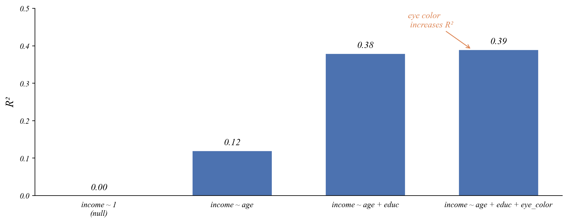
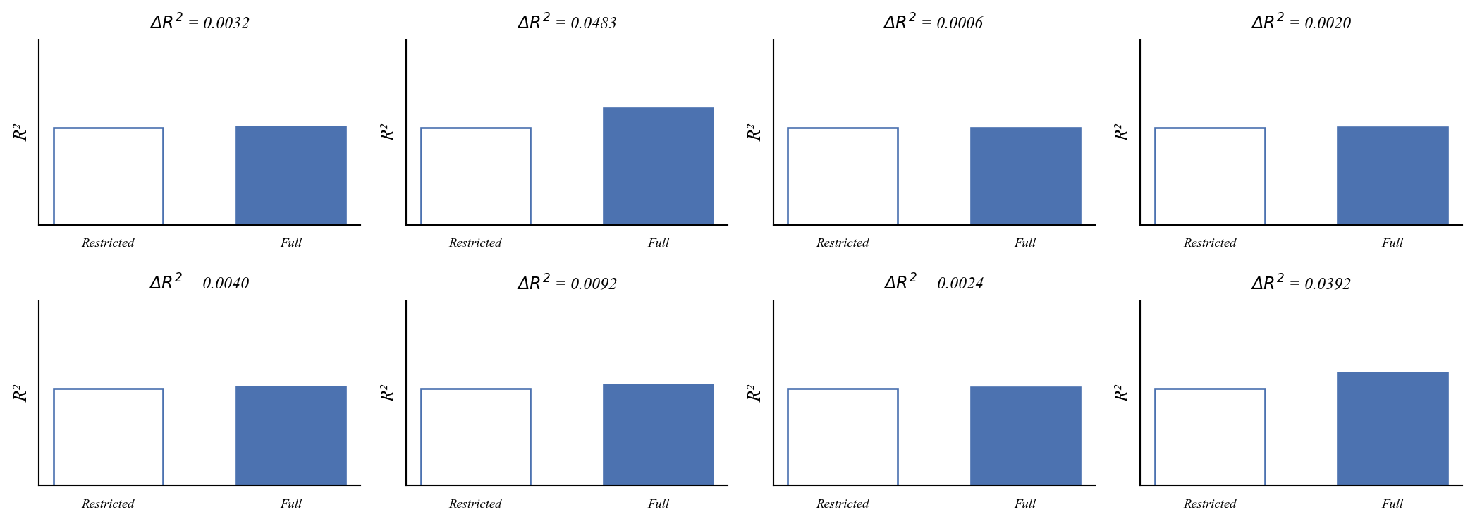
The Problem with R²: Overfitting

R² always goes up when you add variables.

Q. Which of these three models of income do you think is best?

The Problem with R²: Overfitting

R² always goes up when you add variables.

Q. Which of these three models of income do you think is best?

Adding random noise will improve \(R^2\) a little.
Overfitting: the model is fitting the noise, not the signal.
How do we know if the improvement is due to noise?

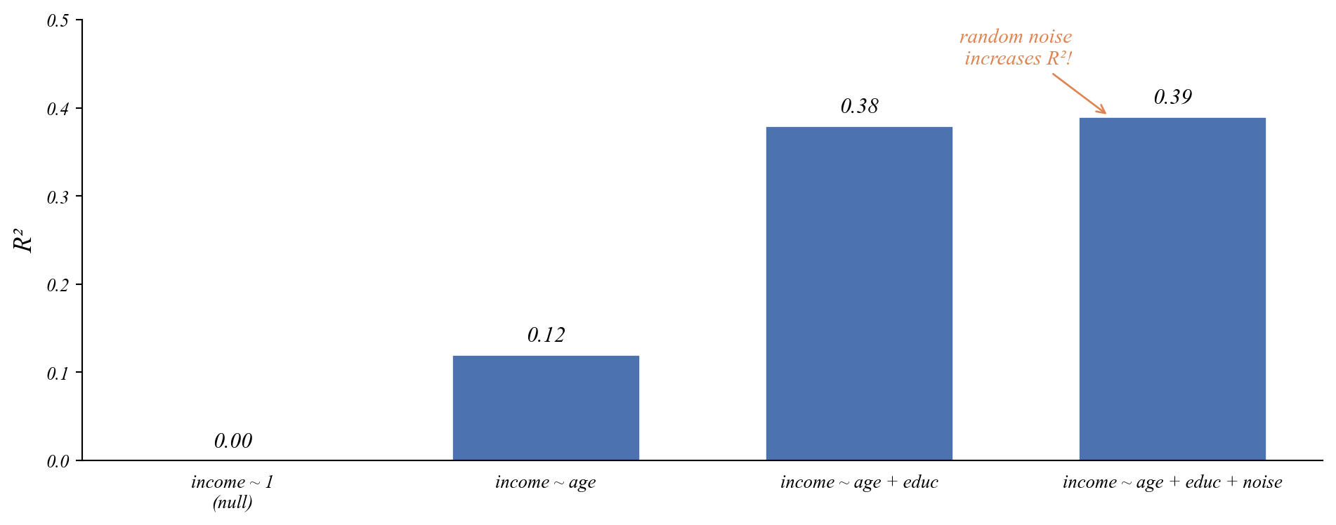
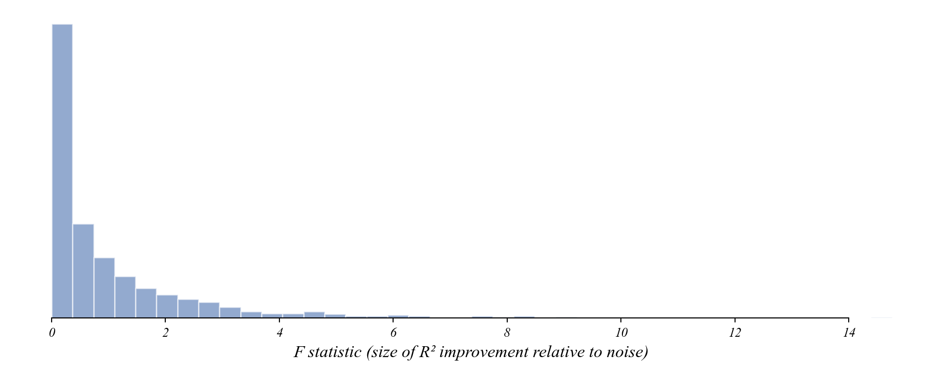
What happens when we add noise?

Lets add two random variables to a model and see what happens to R².

Every time we add noise, R² goes up a little. But only a little.

What happens when we do this 1,000 times?

The distribution of R² improvements from adding noise.

Most improvements are tiny. Large improvements from noise are rare.

The F-statistic

Measuring the size of the R² improvement relative to noise.

\[F = \frac{(R^2_F - R^2_R) / k}{(1 - R^2_F) / (n - p)}\]

\(R^2_R\): R² of the restricted model (fewer variables)
\(R^2_F\): R² of the full model (more variables)
\(k\): number of variables added
\(n - p\): remaining degrees of freedom

Numerator: average R² gain per variable.

Denominator: average unexplained variation.

The F-distribution

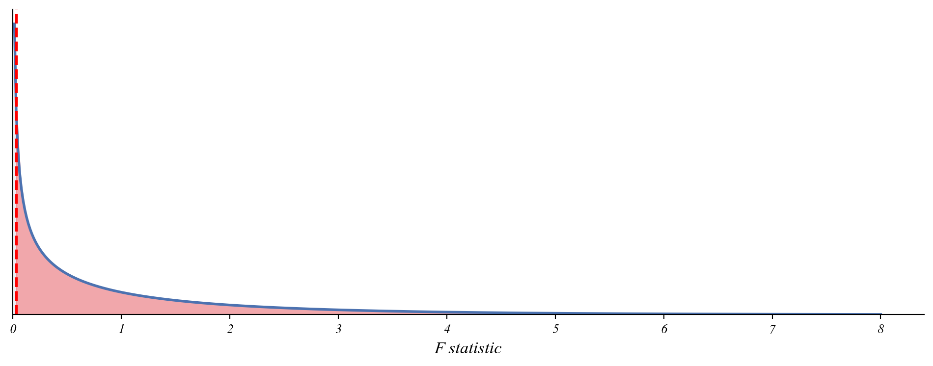
Our simulation matches a known distribution.

The t-distribution described sampling variation in slopes.
The F-distribution describes sampling variation in R² improvements.

Testing Noise

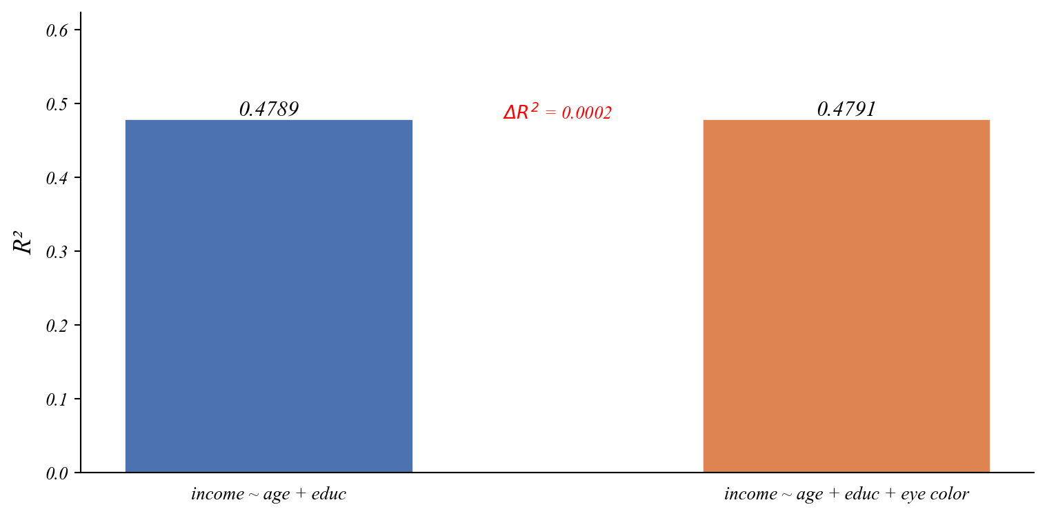
Does adding eye color to the income model improve it?

R² went up. But is this improvement real?

Testing Noise

Where does eye color land on the F-distribution?

F-statistic: 0.03
p-value: 0.857

Large p-value. The improvement is just overfitting.

Testing Noise

Where does eye color land on the F-distribution?

F-statistic: 0.03
p-value: 0.857

Large p-value. The improvement is just overfitting.

We could also check the t-test on the noise coefficient:

==============================================================================
                 coef    std err          t      P>|t|      [0.025      0.975]
------------------------------------------------------------------------------
Intercept      6.8949      4.274      1.613      0.110      -1.590      15.380
age            0.2350      0.063      3.737      0.000       0.110       0.360
educ           1.9802      0.227      8.723      0.000       1.530       2.431
noise          0.1417      0.785      0.180      0.857      -1.417       1.701
==============================================================================

Both the t-test and the F-test agree: noise doesn’t help.

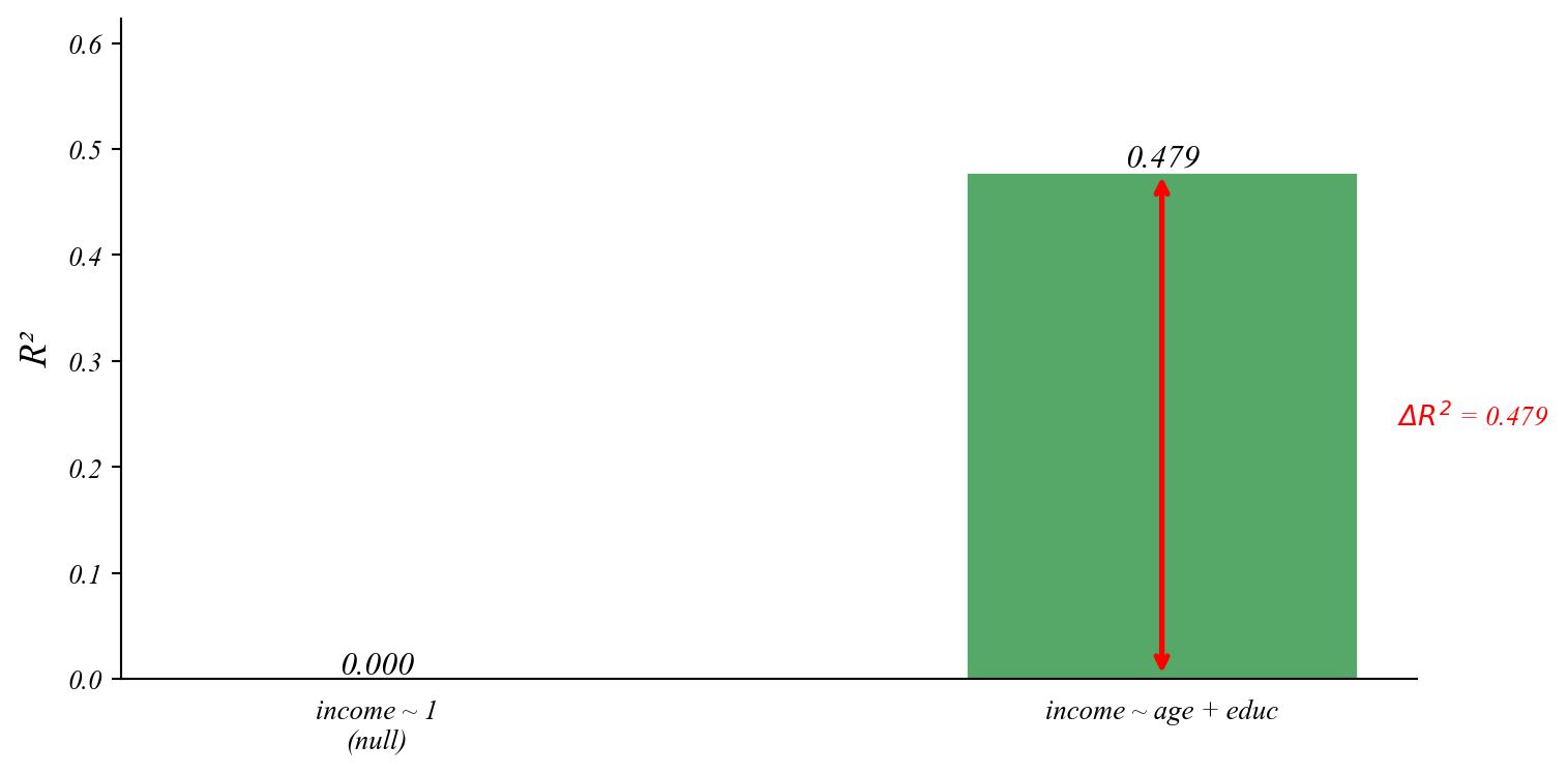
But what about multiple variables?

Can we use the t-test to ask whether age and education jointly improve the model?

The t-test checks one coefficient at a time. It can tell us:

Does age matter? (test \(\beta_1\))
Does education matter? (test \(\beta_2\))

But it can’t tell us: do age and education together improve the model?

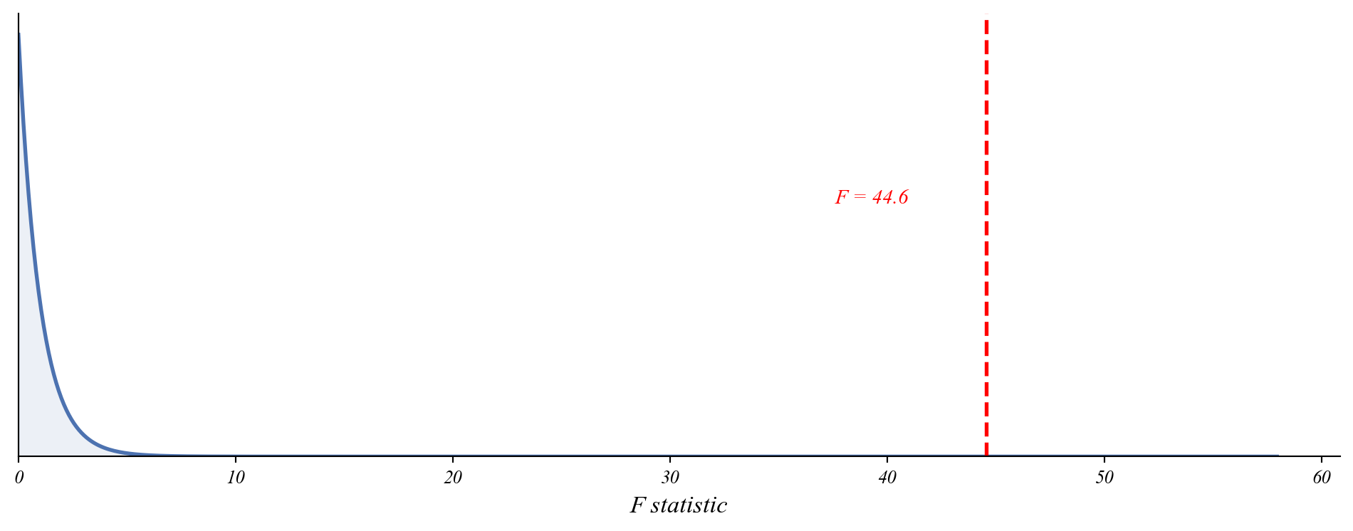
Testing the Full Model

Do age and education together improve predictions?

Testing the Full Model

Where does the full model land on the F-distribution?

F-statistic: 44.58
p-value: 0.000000

Age and education together significantly improve the model.

Model Selection Framework

The research question determines the model.

Question Type	Model
Change in single group	\(y = \beta_0 + \varepsilon\) (One-sample t-test)
Differences between groups	\(y = \beta_0 + \beta_1 Group + \varepsilon\) (Two-sample t-test)
Relationship between vars	\(y = \beta_0 + \beta_1 x + \varepsilon\) (Simple regression)
Multiple factors	\(y = \beta_0 + \beta_1 x_1 + \beta_2 x_2 + \varepsilon\) (Multiple reg)
Group-specific relationships	\(y = \beta_0 + \beta_1 x + \beta_2 Group + \beta_3 x \times Group + \varepsilon\) (Interactions)
Temporal patterns	\(y_t = \beta_0 + \beta_1 t + \beta_2 Season + \varepsilon_t\) (Time series with fixed effects)
Many more!	(You can construct your own)

Practice: Which Model?

For each question, identify the model type and write the equation.

(a) Did average household income change after a new factory opened?

\[\text{income_change} = \beta_0 + \varepsilon\]

(b) Does the effect of study hours on GPA differ for STEM vs. non-STEM majors?

\[\text{GPA} = \beta_0 + \beta_1 \text{hours} + \beta_2 \text{STEM} + \beta_3 \text{hours} \times \text{STEM} + \varepsilon\]

(c) Is there a relationship between commute time and job satisfaction, controlling for salary?

\[\text{satisfaction} = \beta_0 + \beta_1 \text{commute} + \beta_2 \text{salary} + \varepsilon\]

Summary

Main ideas about causation, controls, and model selection

Start with the question — What is the causal story? What confounders exist?
Visualize — Patterns reveal what model to use
Choose the right model — Match the question to the framework
Add controls — Remove potential confounders
Compare models — Use R² and F-tests to evaluate
Interpret with caution — Controls help, but don’t prove causation