ECON 0150 | Economic Data Analysis
The economist’s data analysis pipeline.
Part 5.3 | Numerical Control Variables
Pittsburgh Housing
What is the value of an additional square foot of living area?
House prices depend on:
- Square foot
- Age of the house
- Number of bedrooms
- Neighborhood
- Many other factors!
Pittsburgh Housing
What is the value of an additional square foot of living area?
Pittsburgh housing data with 10,000 homes.
Variables:
SALEPRICE: Sale price of the homeLOGPRICE: Log of sale priceFINISHEDLIVINGAREA: Square footage of finished living spaceYEARBLT: Year the home was built
Pittsburgh Housing: Separate Models
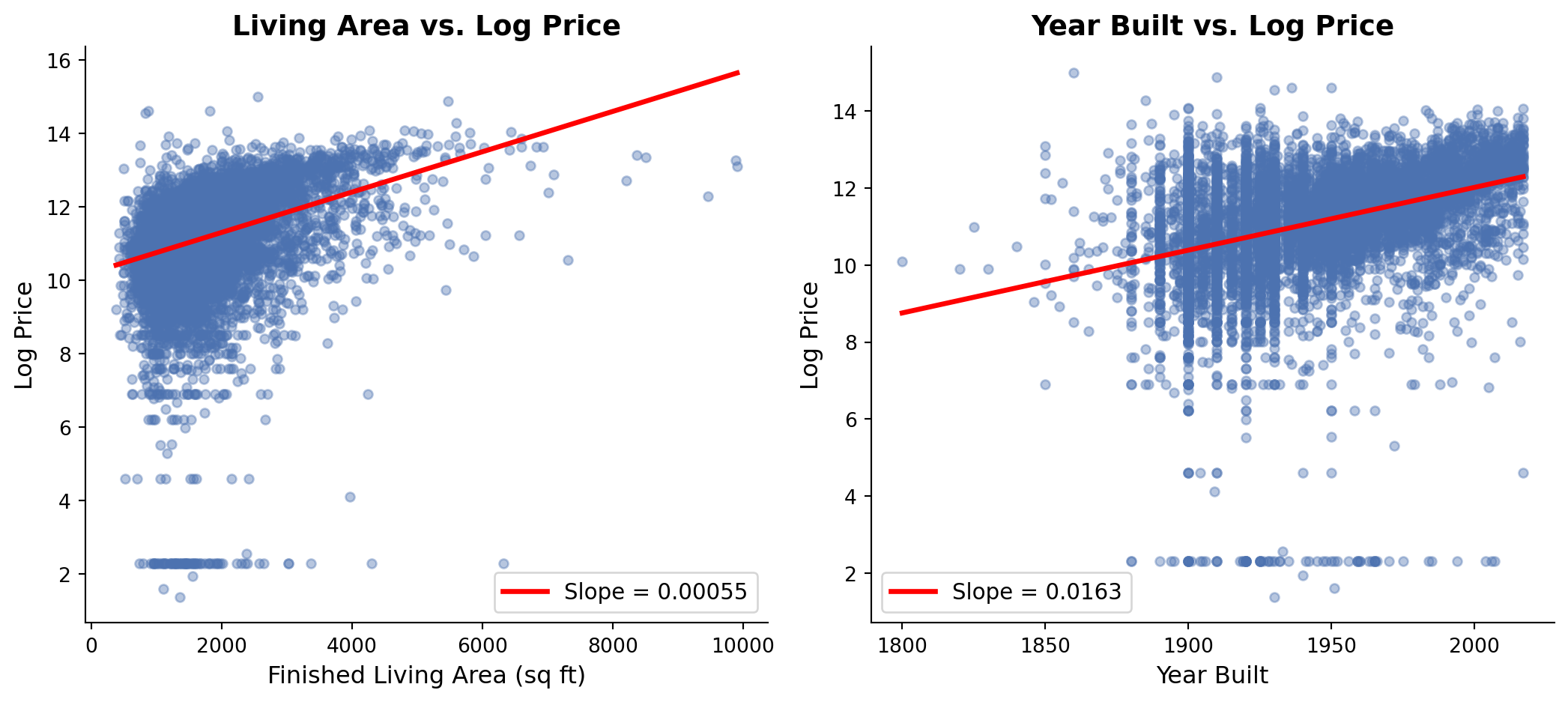
Lets predict price using Living Area and Year Built.
Both living area and year built have positive relationships with price.
Pittsburgh Housing: Related Predictor Variables
Predictor variables Living Area and Year Built are themsevles correlated.
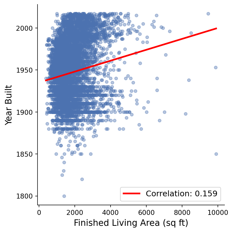
Larger homes tend to be built more recently.
So maybe larger homes are more valuable simply because they’re newer….
Pittsburgh Housing: Multiple Regression
We can model multiple predictor variables simultaneously.
The Multiple Regression Equation
Extending the best-fitting line to multiple dimensions
Single Variable:
\[\text{LogPrice} = \beta_0 + \beta_1 \times \text{LivingArea} + \epsilon\]
Multiple Variables:
\[\text{LogPrice} = \beta_0 + \beta_1 \times \text{LivingArea} + \beta_2 \times \text{YearBuilt} + \epsilon\]
Interpretation:
- \(\beta_0\) = Base log price (intercept)
- \(\beta_1\) = Effect of one more square foot, holding year built constant
- \(\beta_2\) = Effect of being built one year later, holding living area constant
Pittsburgh Housing
What is the value of an additional square foot?
Without controlling for year built:
- We compare small (old) houses to large (new) houses
- The size effect includes the age effect
- Overestimates the true value of square footage
With controlling for year built:
- We compare houses of similar age but different sizes
- Isolates the pure size effect
- Gives us the true value of square footage
This is what we call a control variable.
Multiple Regression with Control
We can adjust for multiple variables simultaneously.
Model 1: Living Area Only
======================================================================================
                         coef    std err          t      P>|t|      [0.025      0.975]
--------------------------------------------------------------------------------------
Intercept             10.2029      0.031    328.476      0.000      10.142      10.264
FINISHEDLIVINGAREA     0.0005   1.65e-05     33.260      0.000       0.001       0.001
======================================================================================


Model 3: Living Area + Year Built Control
======================================================================================
                         coef    std err          t      P>|t|      [0.025      0.975]
--------------------------------------------------------------------------------------
Intercept            -17.9337      0.741    -24.213      0.000     -19.386     -16.482
FINISHEDLIVINGAREA     0.0005   1.56e-05     29.095      0.000       0.000       0.000
YEARBLT                0.0145      0.000     38.018      0.000       0.014       0.015
======================================================================================
Comparing Models
Compare coefficients with and without the control.
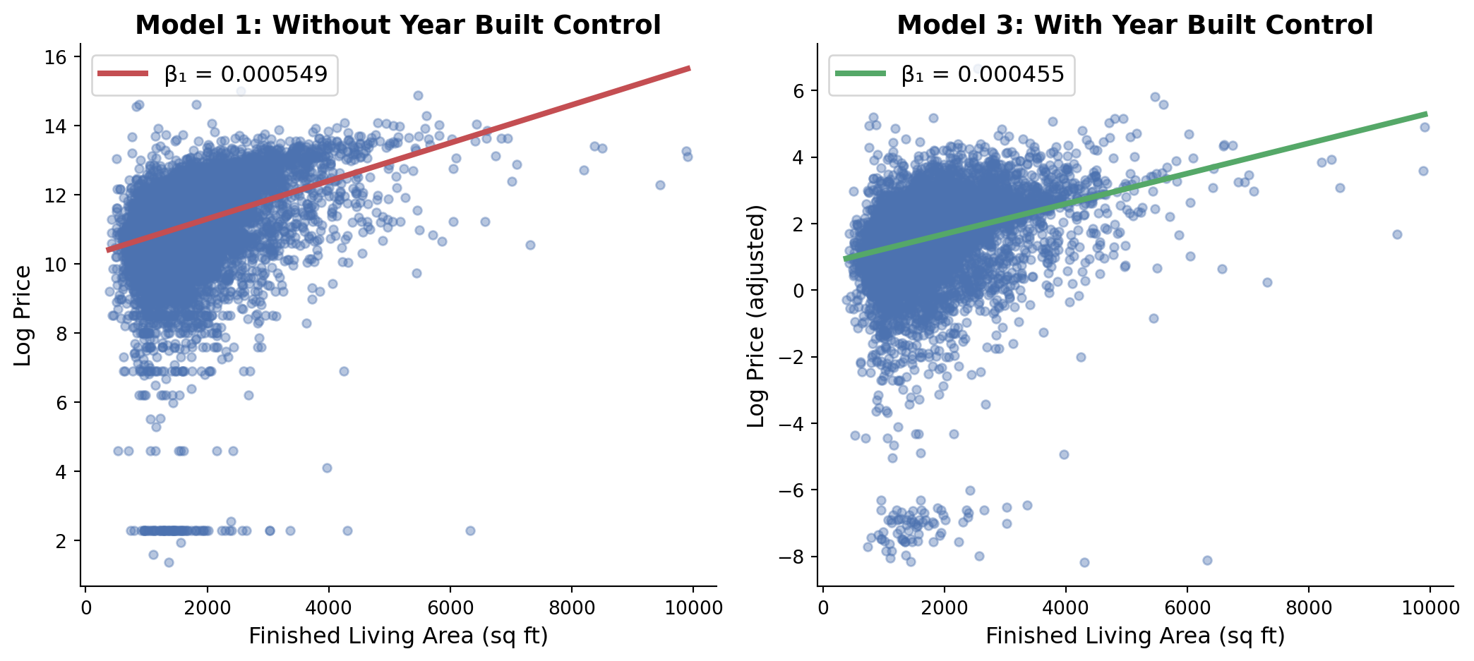
Without control: size effect was inflated by age effect
With control: we get the size effect between houses of equal age
Residual Diagnostics
Checking if our model improved
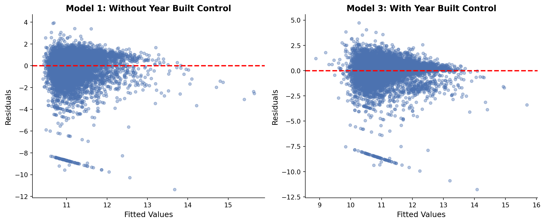
Residuals look somewhat more random with the control.
Log Interpretation
For log outcomes, coefficients represent proportional changes.
For small coefficients (< 0.1):
\[\beta \times 100 \approx \text{percentage change}\]
Interpretation (holding year built constant):
  - Each additional sq ft increases price by 0.045%
  - 100 additional sq ft increases price by 4.55%
Interpretation (holding living area constant):
  - Each year newer increases price by 1.454%
  - A house 10 years newer increases price by 14.54%
The “Holding Constant” Intuition
A control variable compares two similar observations.
Without control (simple regression):
\[\text{LogPrice} = \beta_0 + \beta_1 \times \text{LivingArea} + \epsilon\]
- Compares all small houses to all large houses
- Large houses are newer, so \(\beta_1\) captures both size AND age effects
With control (multiple regression):
\[\text{LogPrice} = \beta_0 + \beta_1 \times \text{LivingArea} + \beta_2 \times \text{YearBuilt} + \epsilon\]
- Compares small and large houses built in the same year
- \(\beta_1\) now captures only the pure size effect
- \(\beta_2\) captures only the pure age effect
Summary
Main ideas about numerical control variables
- Control variables help isolate the effect of your main predictor
- “Holding constant” means comparing observations with similar control values
- Coefficients change when you add controls because you remove confounding
- Choose controls carefully: confounders yes, mediators no
- Check residuals to see if controls improved the model
Exercise 5.3 | Pittsburgh Housing Prices
Lets find the value of an extra square feet in the Pittsburgh housing market.
Step 1: Load and Explore the Data
Step 2: Modeling Relationships Separately
Step 3: Compare Living Area and Year Built
Step 4: Multiple Regression with Control Variable
Step 5: Checking Residuals
# Create residual plots for both models
fig, (ax1, ax2) = plt.subplots(1, 2, figsize=(12, 5))

# Model 1: Without control
residuals_area = model_area.resid
predictions_area = model_area.fittedvalues
ax1.scatter(predictions_area, residuals_area, alpha=0.5, color='#4C72B0')
ax1.axhline(y=0, color='red', linestyle='--', linewidth=2)
ax1.set_title('Model 1: Without Year Built Control')

# Model 3: With control
residuals_both = model_both.resid
predictions_both = model_both.fittedvalues
ax2.scatter(predictions_both, residuals_both, alpha=0.5, color='#4C72B0')
ax2.axhline(y=0, color='red', linestyle='--', linewidth=2)
ax2.set_title('Model 3: With Year Built Control')