ECON 0150 | Economic Data Analysis

The economist’s data analysis skillset.

Part 5.2 | Interaction Models

Model 3: Different Returns to Education

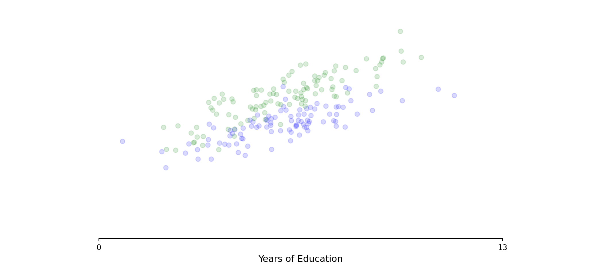
What if education benefits genders differently?

Model 3: Different Returns to Education

What if education benefits genders differently?

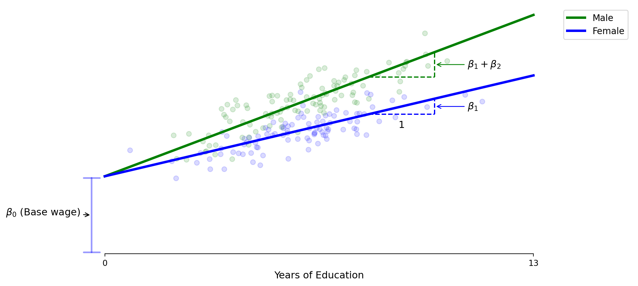
\[\text{Wage} = \beta_0 + \beta_1 \times \text{Education} + \beta_2 \times \text{Education} \times \text{Male} + \varepsilon\]

Model 3: Different Returns to Education

What if education benefits genders differently?

\[\text{Wage} = \beta_0 + \beta_1 \times \text{Education} + \beta_2 \times \text{Education} \times \text{Male} + \varepsilon\]

• β₁ represents the female return to education.
• β₂ represents the additional male return to education (an additional slope)
• Male education effect is β₁ + β₂, creating diverging wage paths

Model 3: The Code

Implementing the education-gender interaction model

# Fit model with interaction between education and sex
model3 = smf.ols('LNINC ~ EDU + EDU:MALE', data=data).fit()
print(model3.summary().tables[1])

• If β₂ > 0 and significant, male return to education is higher
• This model assumes same baseline (intercept) for both genders

Why log income?

A $5,000 raise means different things to different people

• If income is $25,000, that’s a 20% raise
• If income is $200,000, that’s a 2.5% raise

Economists almost always use \(\ln(\text{Income})\) since it puts everyone on the same percentage scale.

Interpreting Log Income

What does log do to our coefficients?

\[\ln(\text{Income}) = \beta_0 + \beta_1 \times \text{Education} + \beta_2 \times \text{Education} \times \text{Male} + \varepsilon\]

With \(\ln(Y)\), we interpret coefficients as percent changes.

• If \(\beta_1 = 0.08\), income is 8% higher with one more year of education.
• If \(\beta_2 = 0.03\), men get an additional 3% per year of education.

Model 4: Full Gender Difference Model

Combining fixed effects and interactions

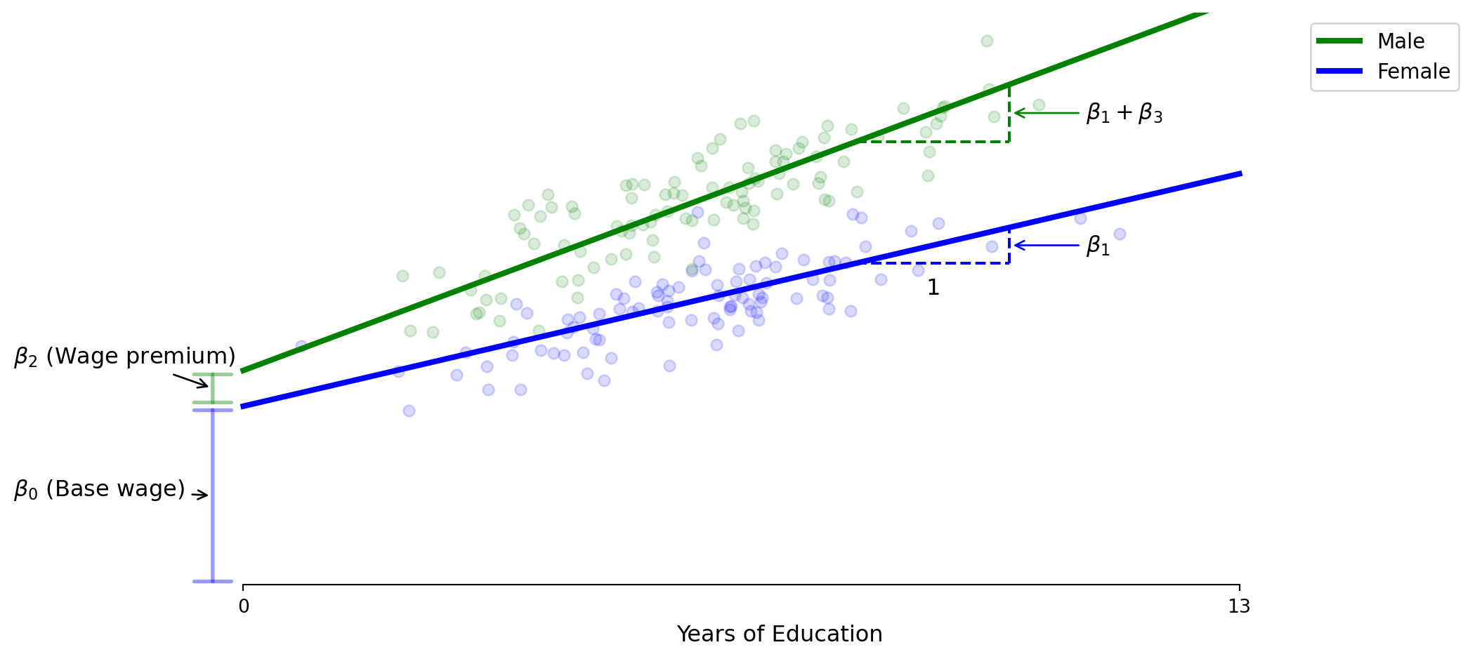
\[\text{Wage} = \beta_0 + \beta_1 \times \text{Education} + \beta_2 \times \text{Male} + \beta_3 \times \text{Education} \times \text{Male} + \varepsilon\]

Model 4: Full Gender Difference Model

Combining fixed effects and interactions

\[\text{Wage} = \beta_0 + \beta_1 \times \text{Education} + \beta_2 \times \text{Male} + \beta_3 \times \text{Education} \times \text{Male} + \varepsilon\]

• β₀ = base wage
• β₂ = initial wage gap (at zero education)
• β₁ = female returns to education
• β₃ = male education return premium

Model 4: The Code

Implementing the full gender difference model

# Fit full model with both sex indicator and interaction
model4 = smf.ols('LNINC ~ EDU + MALE + EDU:MALE', data=data).fit()
print(model4.summary().tables[1])

> allows for differences in both baseline wages and educational returns

Comparison of Models

Different models answer different questions

Model 1: Fixed Effect

• Question: “Is there a gender wage gap?”

Model 2: Fixed Effect with Control

• Question: “Is there a gender wage gap controling for education?”

Model 3: Interaction Only

• Question: “Are there differences in returns to education?”

Model 4: Fixed Effect and Interaction

• Question: “Does the gender wage gap vary with education level?”

Key Takeaways

General linear model for analyzing group differences

Part 5.1 | Categorical Controls (‘Fixed Effects’)

• Captures level differences between groups

Part 5.2 | Interactions

• Capture differences in slopes

Model Choice should be guided by your research question