ECON 0150 | Economic Data Analysis

The economist’s data analysis skillset.


Part 5.1 | Categorical Controls

Two Hospitals

Which hospital would you choose?

Hospital A has a higher survival rate, seems like the obvious choice.

Two Hospitals

Hospital A looks better…

But is this the whole story?

Two Hospitals

Which hospital would you choose?

What if we break down survival rate by case severity?

Two Hospitals

Hospital B is better in both groups!

Mild cases: B has 98% vs A has 95%

Severe cases: B has 60% vs A has 50%

The Hidden Variable

Why does this happen?

Hospital A treats mostly mild cases, Hospital B treats mostly severe cases.

Simpson’s Paradox

A trend in aggregated data reverses when the data is split into groups.


  • Hospital A appears better overall (86% vs 68%)
  • But Hospital B is better for both mild AND severe cases
  • The confounding variable (patient severity) drives the reversal
  • The hospitals serve different patient populations

The Lesson

Why we need to control for other variables


  • Aggregate statistics can be misleading
  • Hidden variables can confound relationships
  • To understand true effects, we need to control for confounders
  • That’s what Part 5 is about: adding controls to our models

GLM: The Gender Wage Gap

Lets use the general linear model to test for differences in wages by gender.


Questions:

  • Is there a wage gap between male / female?
  • Are returns to education different between male / female?

Model 1: Basic Gender Wage Gap

The simplest model with just a gender indicator.

Model 1: Basic Gender Wage Gap

The simplest model with just a gender indicator.

\[\text{Wage} = \beta_0 + \beta_1 \times \text{Male} + \varepsilon\]

Model 1: Basic Gender Wage Gap

The simplest model with just a gender indicator.

\[\text{Wage} = \beta_0 + \beta_1 \times \text{Male} + \varepsilon\]

  • β₀ is the average wage for female
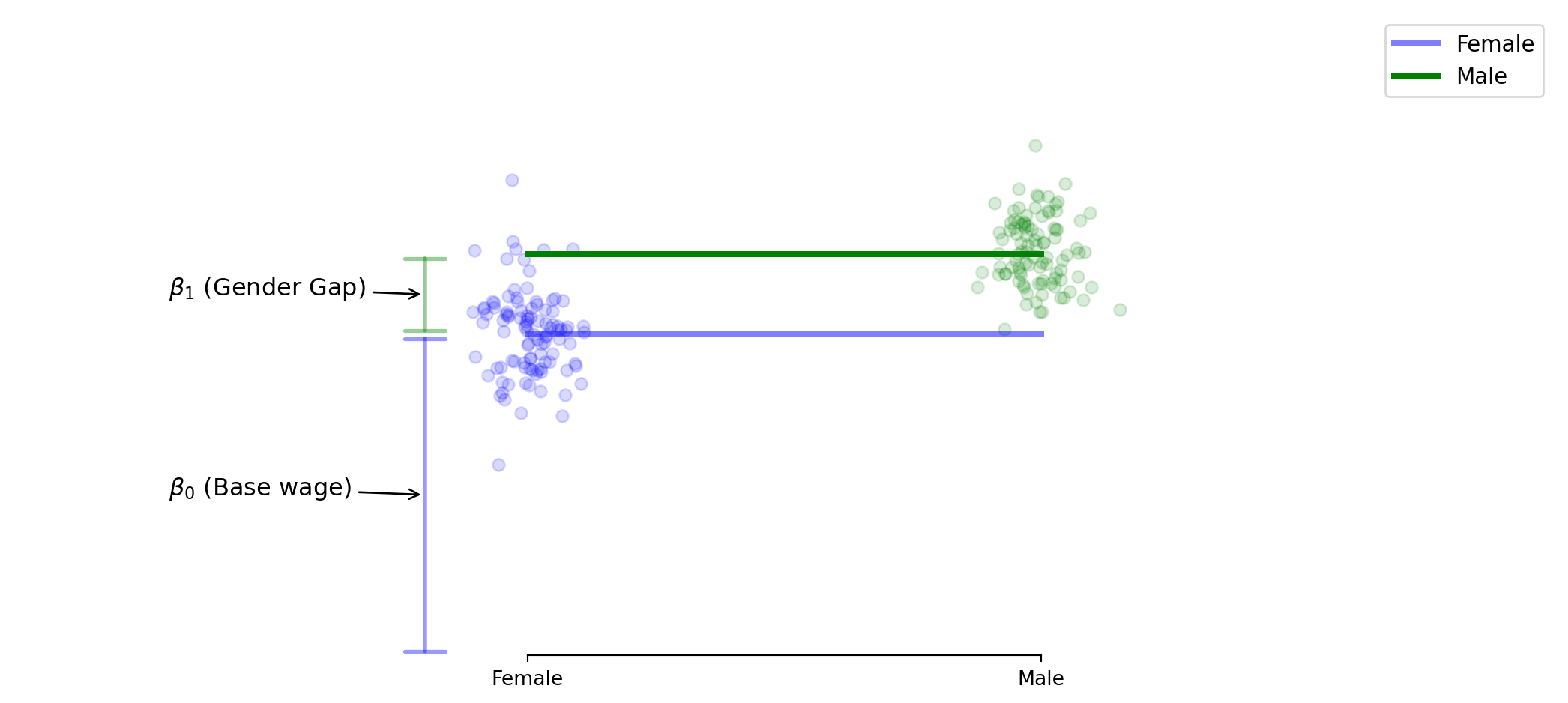
  • β₁ represents the gender wage gap, the additional wage for male
  • We often call a Categorical Control variable like this a “Fixed Effect”

Model 1: The Code

Implementing the basic gender gap model

import statsmodels.formula.api as smf

# Fit the model with just the male indicator
model1 = smf.ols('INCLOG10 ~ MALE', data=data).fit()
print(model1.summary().tables[1])


  • If β₁ > 0, this is evidence of a difference in income by gender
  • There are many possible explainations for this gap
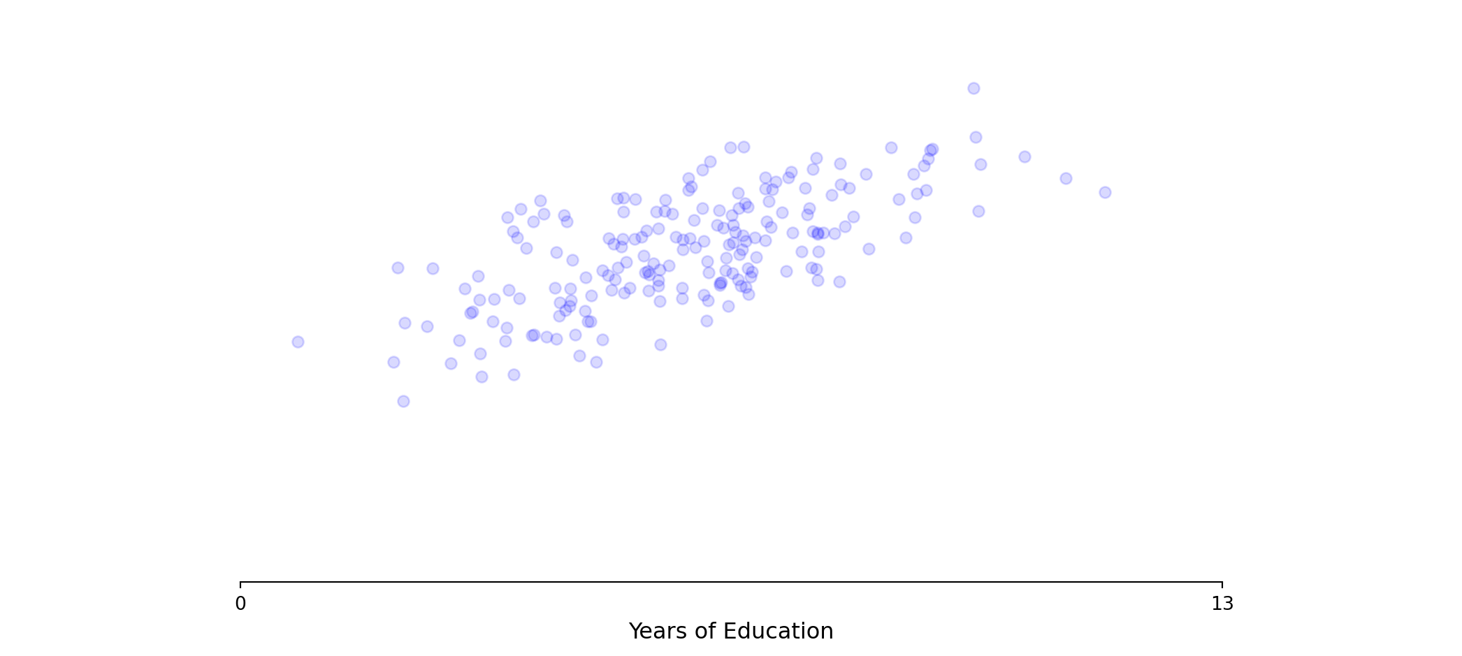
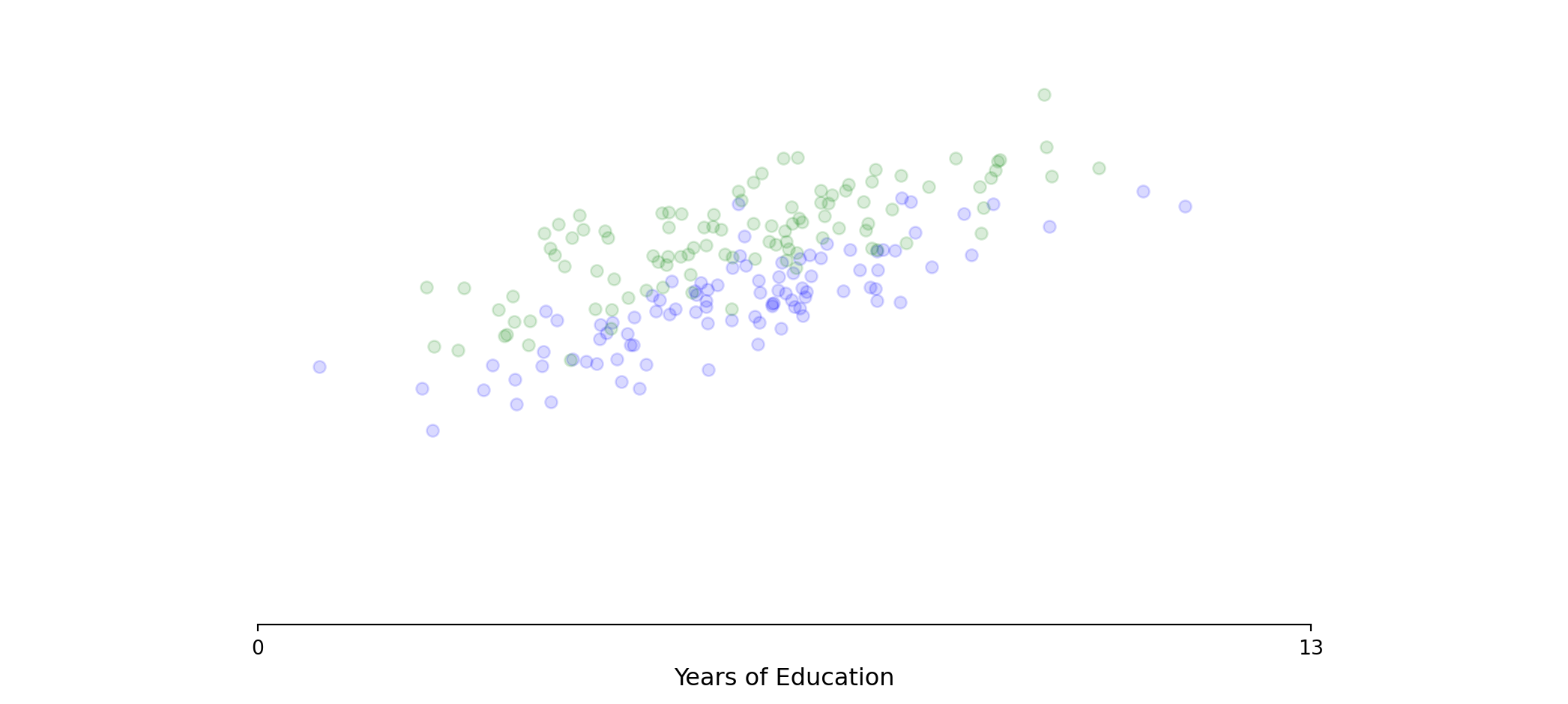
  • What if the gap is related to some other factor (eg. education)?

Model 2: Education + Gender Wage Gap

Adding education as a control variable.

Model 2: Education + Gender Wage Gap

Adding education as a control variable.

Model 2: Education + Gender Wage Gap

Adding education as a control variable.

\[\text{Wage} = \beta_0 + \beta_1 \times \text{Education} + \beta_2 \times \text{Male} + \varepsilon\]

Model 2: Education + Gender Wage Gap

Adding education as a control variable.

\[\text{Wage} = \beta_0 + \beta_1 \times \text{Education} + \beta_2 \times \text{Male} + \varepsilon\]

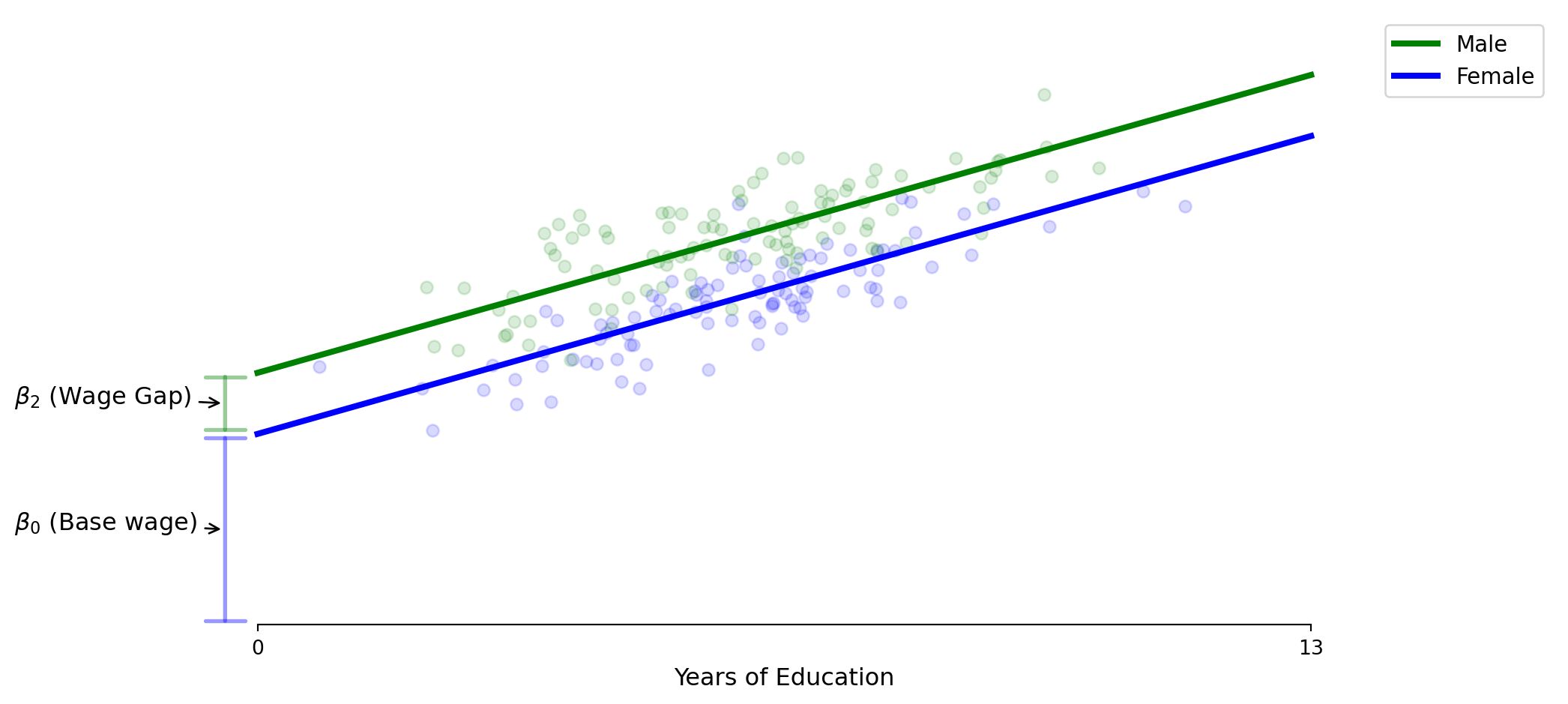
> β₀ is the base wage for those with no post-middle school education

> β₂ represents the gender wage gap, added to the intercept for male only

> model assumes parallel lines, same returns to education (β₁) for everyone

Model 2: The Code

Implementing the gender fixed effect model

import statsmodels.formula.api as smf

# Fit the model with male indicator
model2 = smf.ols('INCLOG10 ~ EDU + MALE', data=data).fit()
print(model2.summary().tables[1])


  • If β₂ > 0, there is evidence of a gender wage gap.

Summary: Categorical Controls

What we learned in Part 5.1


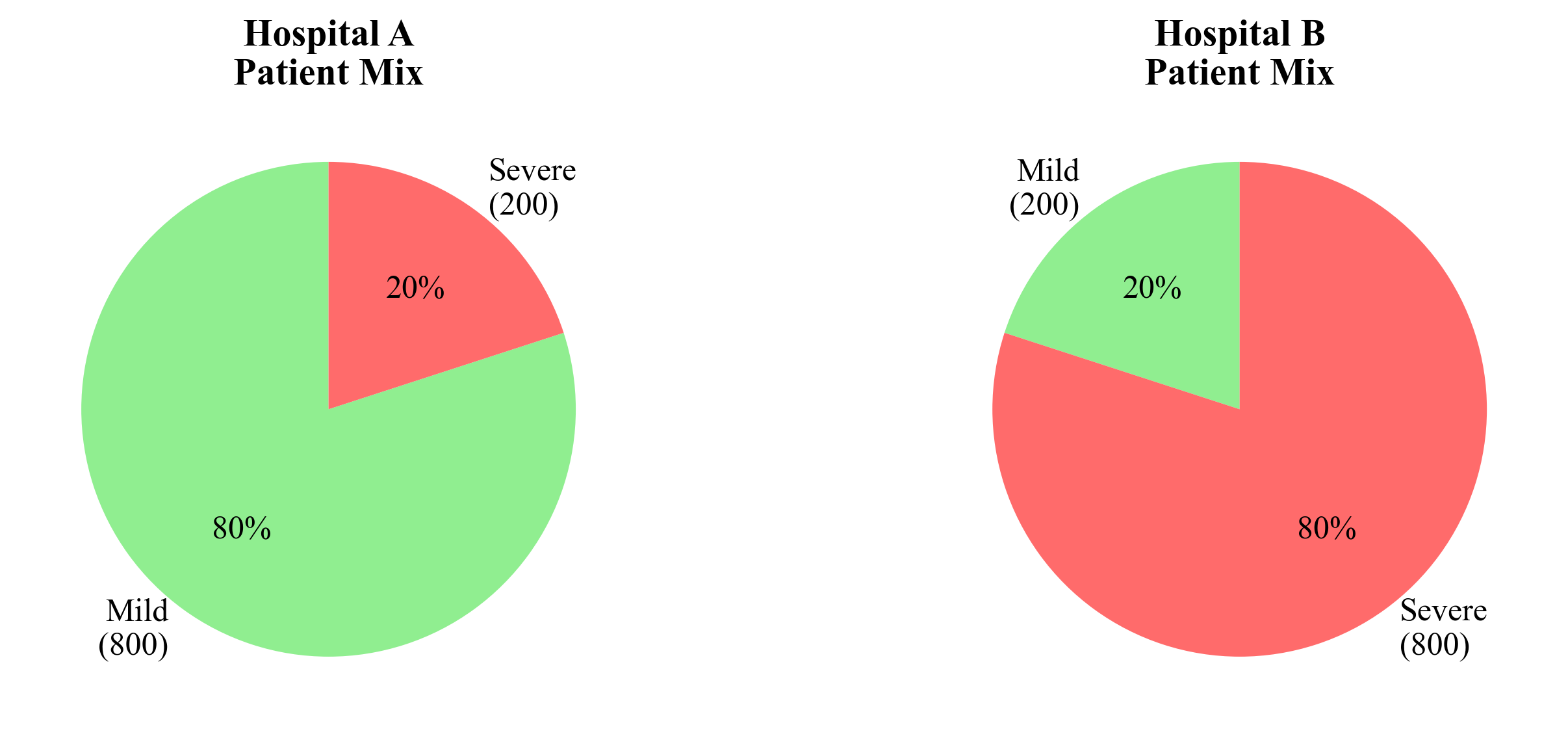
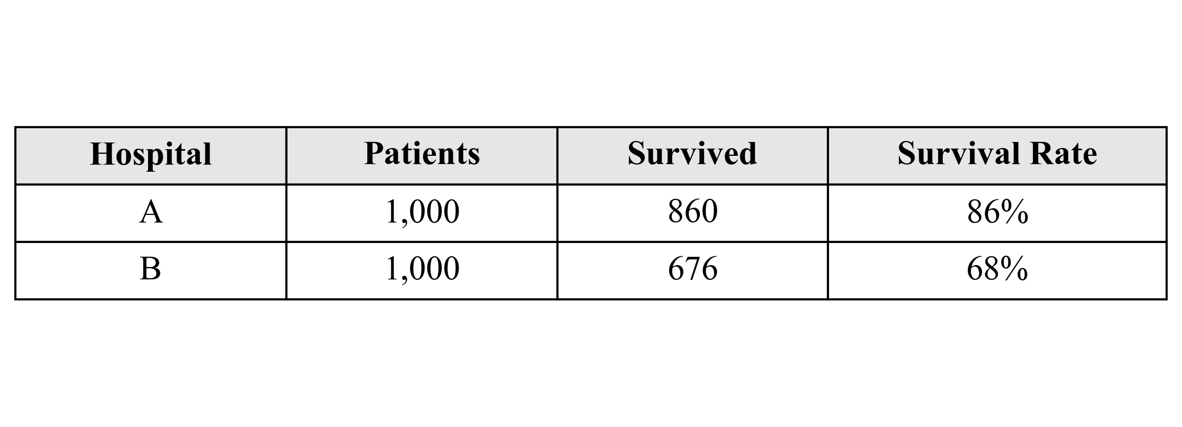
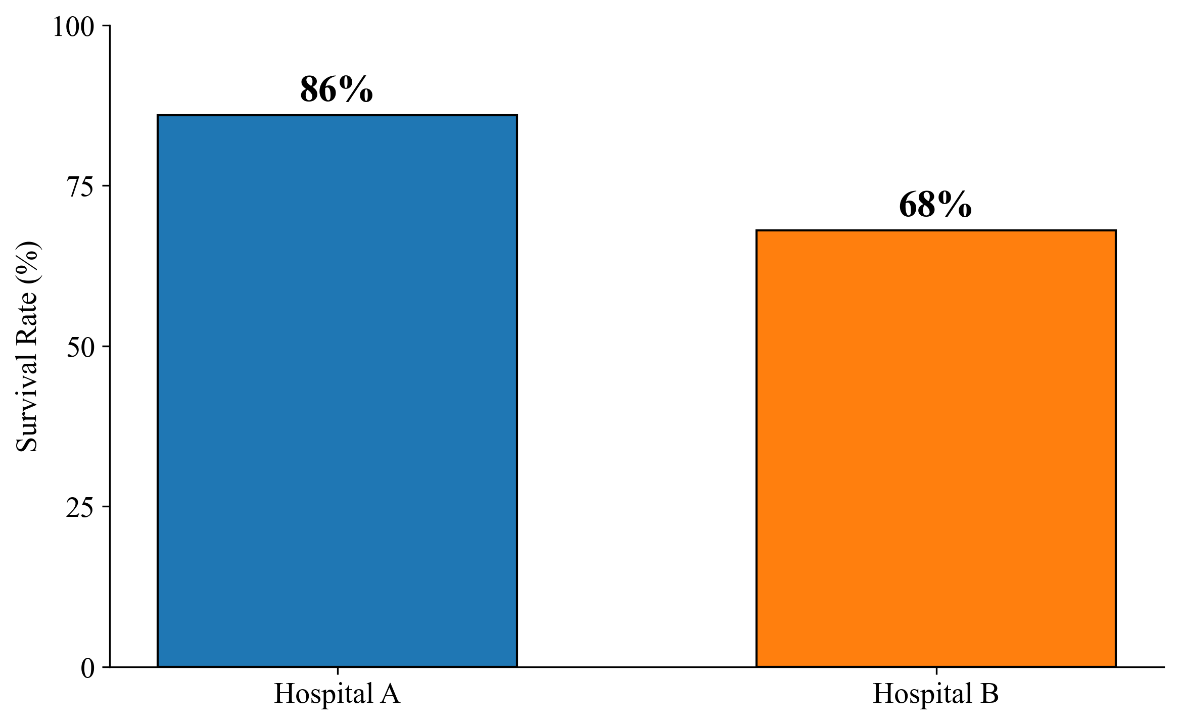
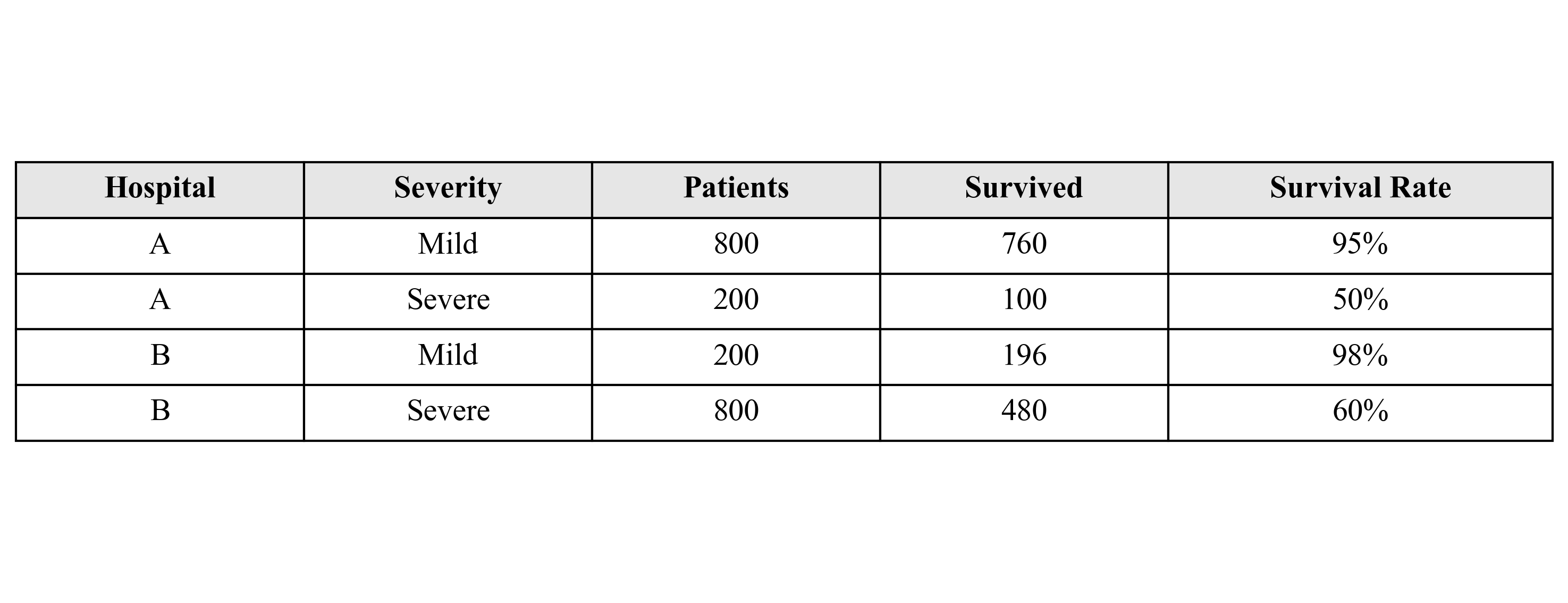
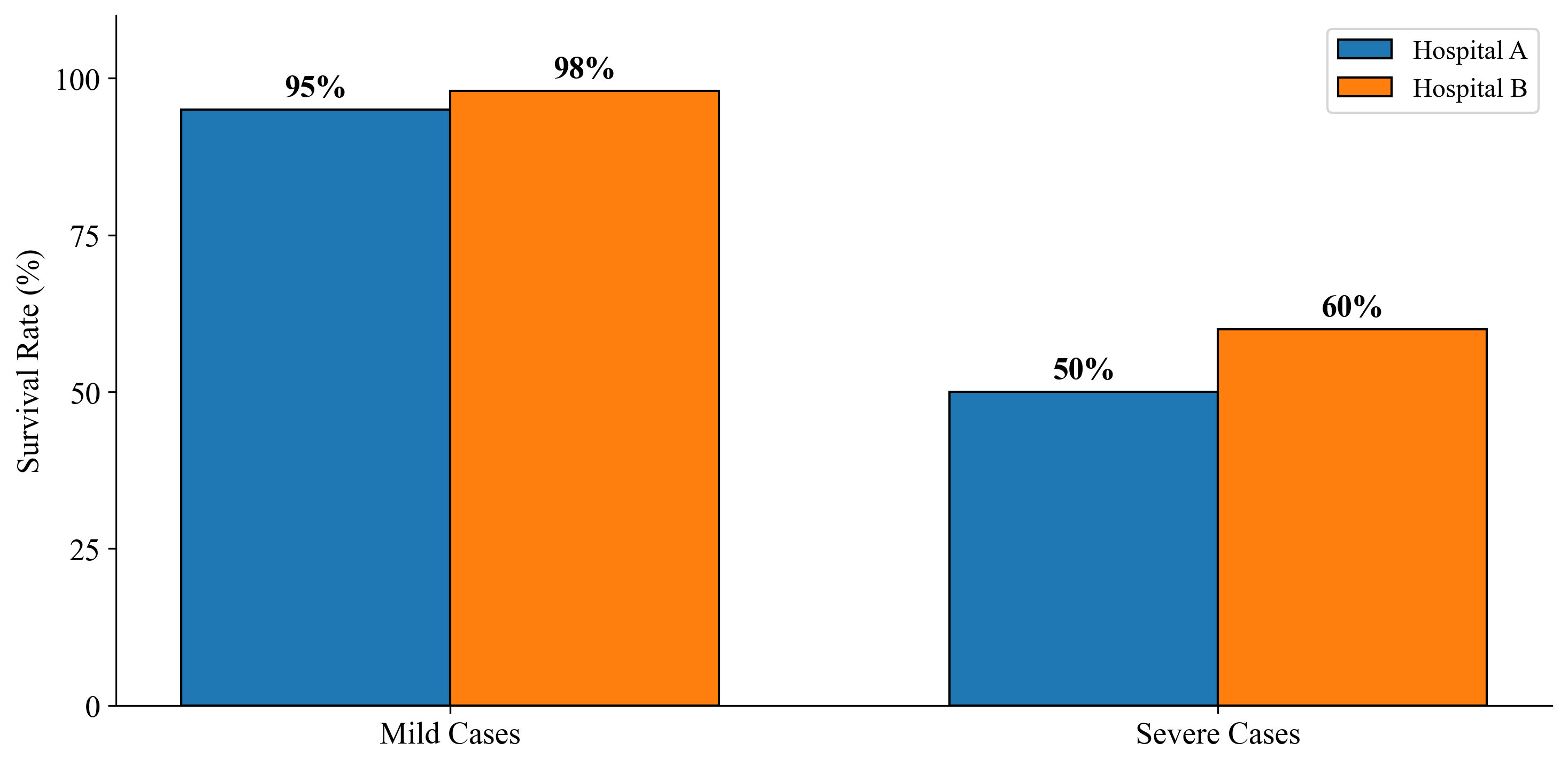
  • Simpson’s Paradox shows why we need to control for confounding variables
  • Categorical controls (fixed effects) capture level differences between groups
  • Model 1: Just the indicator: tests for differences
  • Model 2: Indicator + continuous variable: parallel lines with different intercepts
  • Next: What if the slopes differ between groups?: Part 5.2 Interactions