ECON 0150 | Economic Data Analysis
Part 4 | Review
Part 4: What we’ve learned
- 4.1 Numerical predictors: \(y = \beta_0 + \beta_1 x + \varepsilon\)
- 4.2 Categorical predictors: same equation, \(x\) is 0 or 1
- 4.3 Model assumptions: linearity, homoskedasticity, independence, normality
- 4.4 The problem of timeseries: autocorrelation and differencing
Today: practice problems in the style of the MiniExam.
Practice 1: Numerical predictor
| 0 |
6 |
39.7 |
| 1 |
14 |
26.9 |
| 2 |
11 |
25.6 |
| 3 |
9 |
31.1 |
| 4 |
2 |
40.5 |
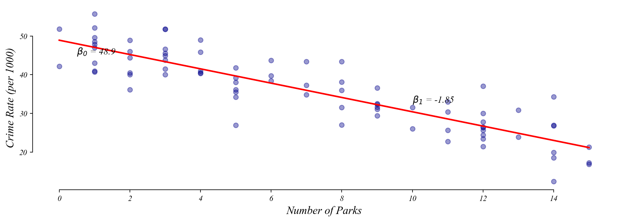
a) How would you visualize the relationship between these two variables?
Scatterplot: num_parks on the x-axis, crime_rate on the y-axis.
b) Write down a model to test whether more parks means lower crime.
\[\text{crime_rate} = \beta_0 + \beta_1 \cdot \text{num_parks} + \varepsilon\]
Practice 1: Numerical predictor
c) What part of your model would indicate a relationship exists?
If \(\beta_1\) is significantly different from zero (small p-value), there is a relationship.
Practice 2: Binary predictor
| 0 |
0 |
39.7 |
0 |
| 1 |
0 |
26.9 |
0 |
| 2 |
0 |
25.6 |
0 |
| 3 |
0 |
31.1 |
0 |
| 4 |
0 |
40.5 |
0 |
a) What is the variable type of has_park?
Binary categorical (0 or 1).
b) Visualize the relationship between has_park and crime_rate.
Strip plot or box plot with has_park on the x-axis and crime_rate on the y-axis.
Practice 2: Binary predictor
c) Write down the model. What does \(\beta_0\) represent? What does \(\beta_1\) represent?
\[\text{crime_rate} = \beta_0 + \beta_1 \cdot \text{has_park} + \varepsilon\]
\(\beta_0\) = Mean crime rate in neighborhoods without parks (x = 0).
\(\beta_1\) = Difference in mean crime rate (has park minus no park).
Practice 2: Binary predictor
d) If we instead coded no_park = 1 for no park, 0 for has park, what changes?
- \(\beta_0\) becomes the mean crime rate for neighborhoods with parks
- \(\beta_1\) flips sign (same magnitude, opposite direction)
\(\beta_0\) is ALWAYS the mean of the group coded as 0.
\(\beta_1\) is ALWAYS the difference (group 1 minus group 0).
Practice 3: Reading regression output
\[\text{test_score} = \beta_0 + \beta_1 \cdot \text{hours_sleep} + \varepsilon\]
                 coef    std err          t      P>|t|      [0.025      0.975]
------------------------------------------------------------------------------
Intercept       42.30      5.100      8.294      0.000      32.22      52.38
hours_sleep      5.80      0.720      8.056      0.000       4.38       7.22
------------------------------------------------------------------------------
a) Interpret the intercept (42.30) in context.
A student who sleeps 0 hours is predicted to score 42.3 points. (Not meaningful.)
b) Interpret the slope (5.80) in context.
Each additional hour of sleep is associated with a 5.8 point increase in test score.
Practice 3: Reading regression output
\[\text{test_score} = \beta_0 + \beta_1 \cdot \text{hours_sleep} + \varepsilon\]
                 coef    std err          t      P>|t|      [0.025      0.975]
------------------------------------------------------------------------------
Intercept       42.30      5.100      8.294      0.000      32.22      52.38
hours_sleep      5.80      0.720      8.056      0.000       4.38       7.22
------------------------------------------------------------------------------
c) What is the null hypothesis for the slope coefficient?
\(H_0: \beta_1 = 0\) or hours of sleep has no effect on test scores.
d) What test score would the model predict for a student who sleeps 8 hours?
\(\hat{y} = 42.3 + 5.8 \times 8 = 88.7\) points.
Practice 4: Drawing the sampling distribution
                 coef    std err          t      P>|t|      [0.025      0.975]
------------------------------------------------------------------------------
Intercept       12.50      1.200     10.417      0.000      10.13      14.87
experience       0.75      0.478      1.570      0.120      -0.20       1.70
------------------------------------------------------------------------------
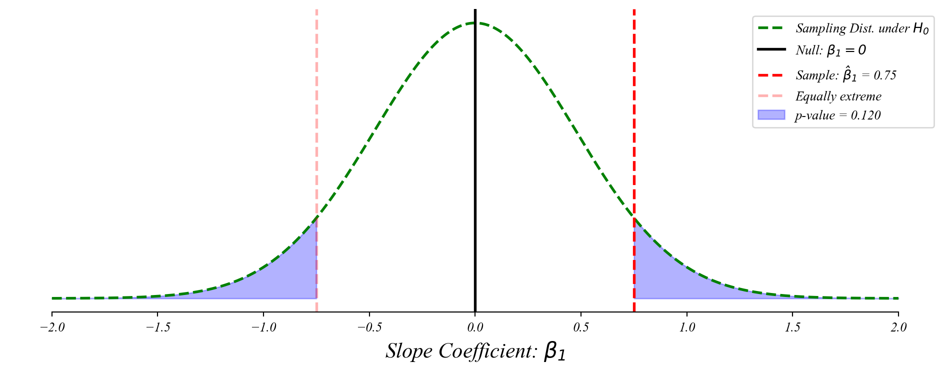
a) Draw the sampling distribution of \(\beta_1\) under the null hypothesis.
Practice 4: Drawing the sampling distribution
- Draw a bell curve centered at 0 (the null hypothesis)
- Label the x-axis: “Slope Coefficient: \(\beta_1\)”
- Mark where 0 is (the null) with a solid line
- Mark where your observed slope is with a dashed line
- Shade the area beyond your observed slope (both tails) is the p-value
Practice 5: Binary predictor
| 0 |
0 |
3.09 |
| 1 |
0 |
2.99 |
| 2 |
0 |
2.54 |
| 3 |
1 |
2.91 |
| 4 |
1 |
2.61 |
a) If we code on_campus = 1 for yes, 0 for no, what does \(\beta_0\) represent?
Mean GPA for off-campus students (the x = 0 group).
b) What does \(\beta_1\) represent?
Difference in mean GPA: on-campus minus off-campus.
Practice 5: Binary predictor
c) Now code off_campus = 1 for off-campus, 0 for on-campus. What changes?
- \(\beta_0\) becomes the mean GPA for on-campus students
- \(\beta_1\) flips sign (same magnitude, opposite direction)
\(\beta_0\) is ALWAYS the mean of the group coded as 0.
\(\beta_1\) is ALWAYS the difference (group 1 minus group 0).
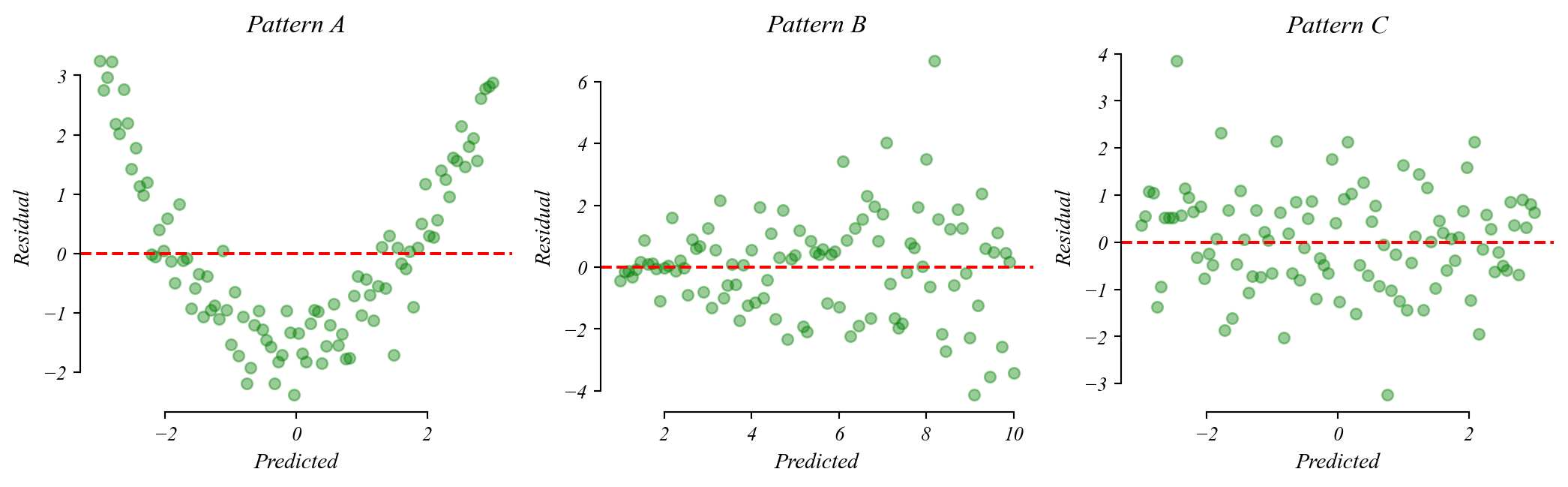
Practice 6: Reading a residual plot
- Pattern A: U-shaped residuals \(\rightarrow\) linearity violated (relationship is curved)
- Pattern B: Fan shape \(\rightarrow\) homoskedasticity violated (variance increases)
- Pattern C: Random scatter \(\rightarrow\) assumptions look fine
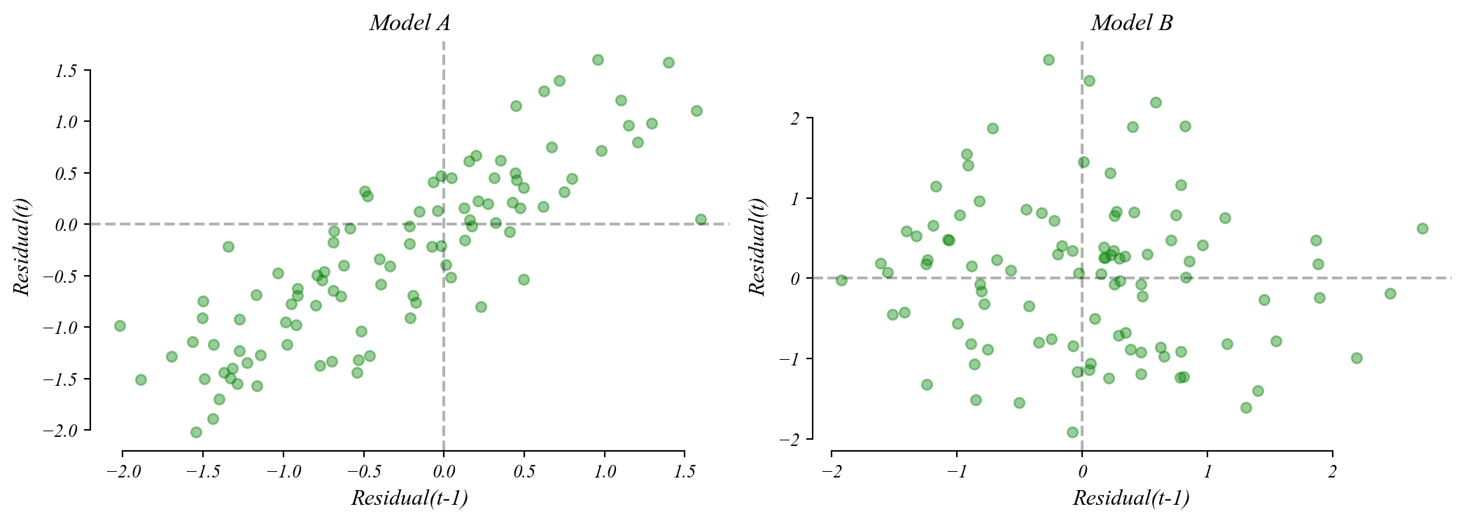
Practice 7: Lagged residual plots
- Model A: Strong positive slope \(\rightarrow\) residuals are autocorrelated (independence violated)
- Model B: Random cloud \(\rightarrow\) residuals are independent (assumption satisfied)
Autocorrelation means the model’s errors follow a pattern over time. Standard errors become unreliable.
Quick reference: what to know for the MiniExam
- Write the model: \(y = \beta_0 + \beta_1 x + \varepsilon\) (works for numerical AND binary \(x\))
- Interpret \(\beta_0\): predicted \(y\) when \(x = 0\) (baseline/reference group)
- Interpret \(\beta_1\): change in \(y\) for a one-unit increase in \(x\) (or difference between groups)
- Sampling distribution: bell curve centered on null, shade tails beyond observed slope
- P-value: probability of observing a slope as extreme as ours if \(\beta_1 = 0\)
- Residual plots: random = good; U-shape = non-linearity; fan = heteroskedasticity
- Lag plots: slope = autocorrelation (independence violated)