ECON 0150 | Economic Data Analysis
Part 4.4 | The Problem of Timeseries
Part 4.3 Recap
Linearity : The relationship between X and Y is linearHomoskedasticity : Equal error variance across all values of XIndependence : Observations are independent from each otherNormality : Errors are normally distributed
Today we focus on Assumption 3: Independence : the problem of timeseries.
Timeseries Analysis
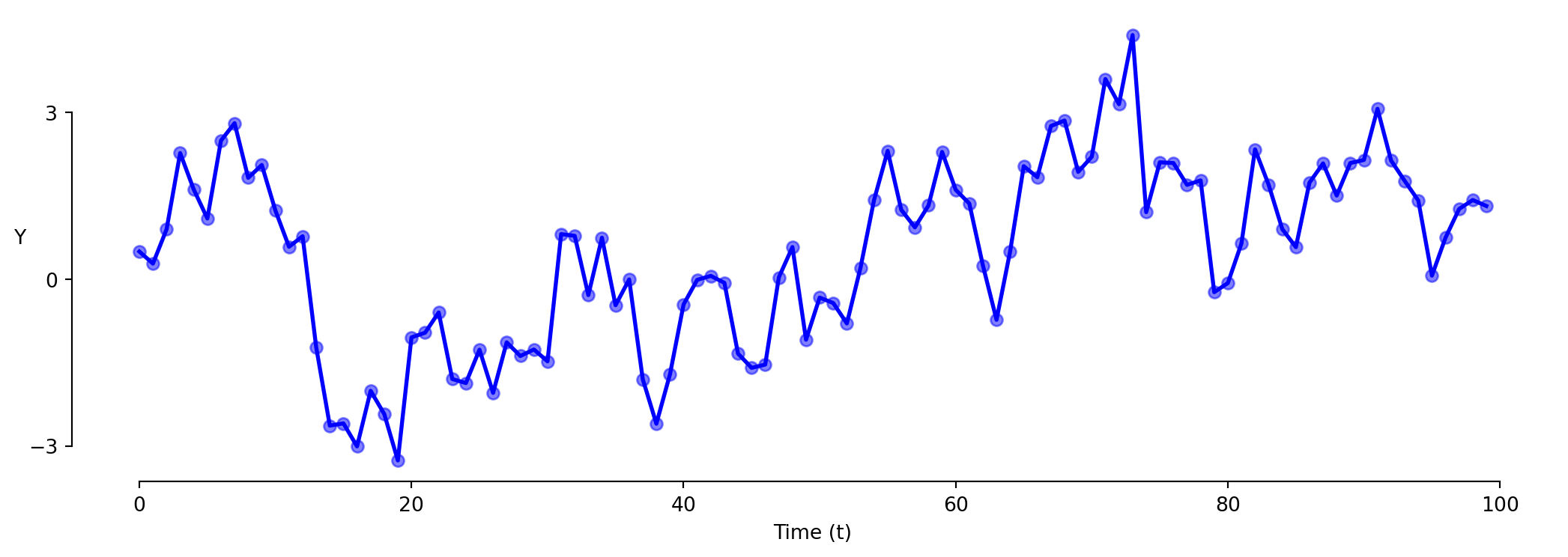
Data related in time has a special problem:
Observations are related to their past values (autocorrelation).
This violates Assumption 4: Independence .
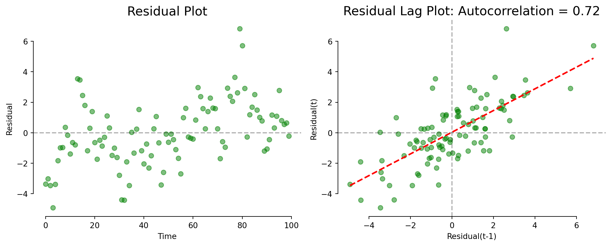
Timeseries Analysis: Autocorrelation
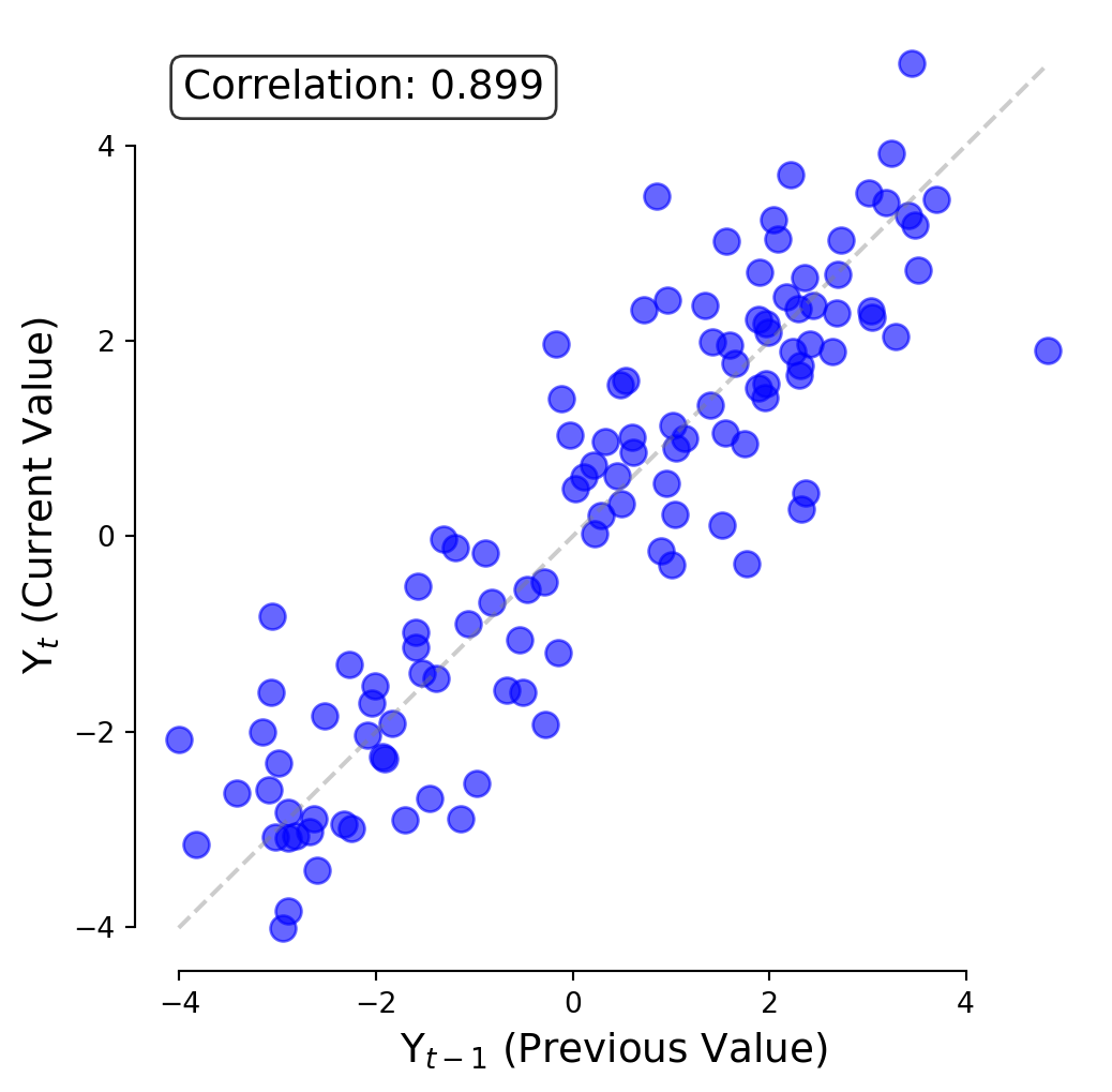
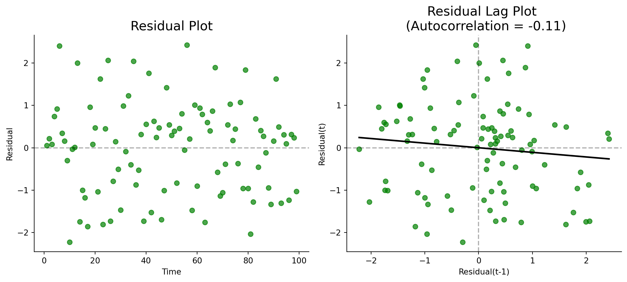
A Lag Plot shows the value today (\(t\) ) against the value yesterday (\(t-1\) ).
Autocorrelation tells us whether today’s value depends on yesterday’s value.
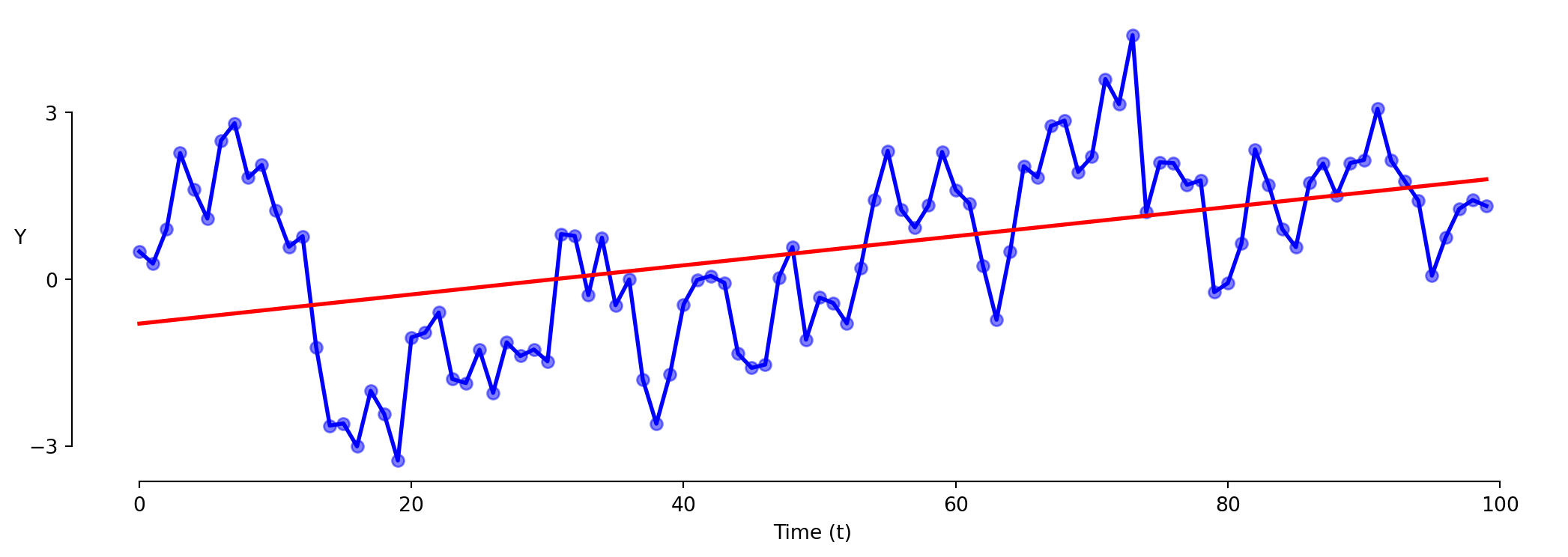
Timeseries: Model 1 (Levels)
\[\text{Y} = \beta_0 + \beta_1 \cdot \text{t} + \varepsilon\]
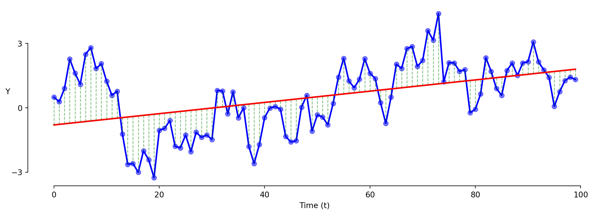
Timeseries: Model 1 (Levels)
\[\text{Y} = \beta_0 + \beta_1 \cdot \text{t} + \varepsilon\]
This model is often wrong in the same direction repeatedly.
Timeseries: Model 1 (Levels)
\[\text{Y} = \beta_0 + \beta_1 \cdot \text{t} + \varepsilon\]
Exercise 4.4 | Model 1 (Levels)
# 1. Fit the levels model = smf.ols('gdp ~ unemployment' , data= data).fit()print (model1.summary().tables[1 ])
# 2. Residual plot 0 , color= 'red' )
# 3. Lagged residual plot - 1 ], model1.resid[1 :])
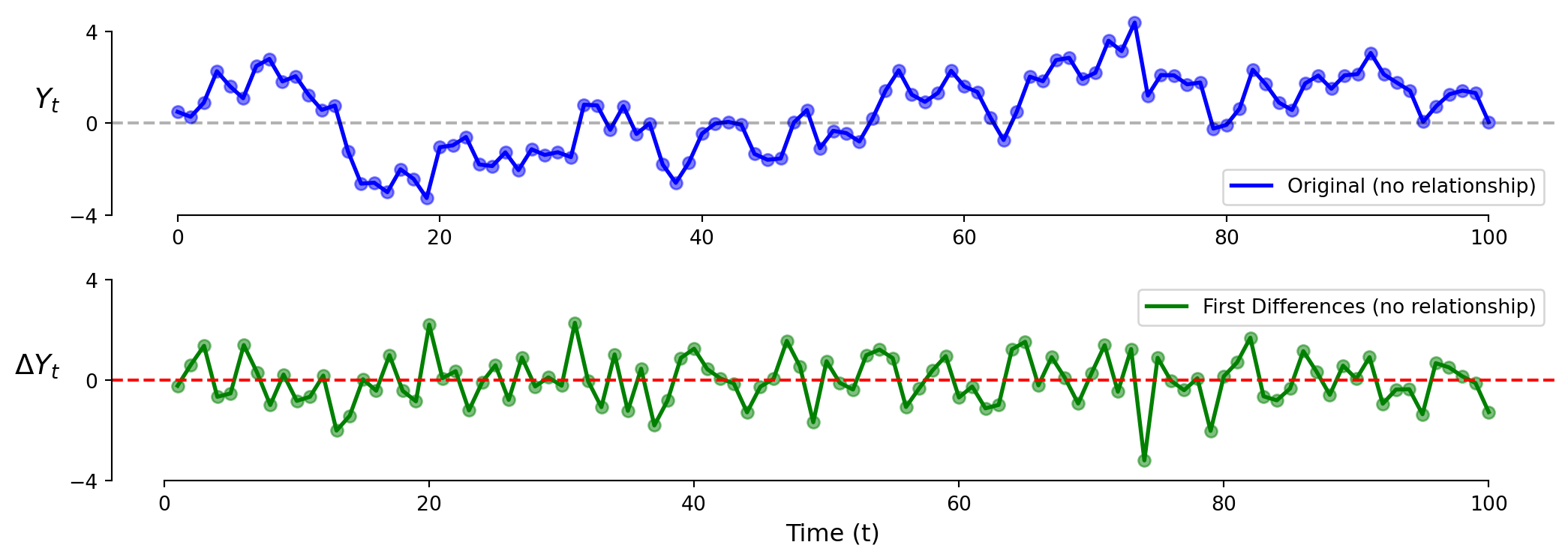
Timeseries: Model 2 (First Differences)
\[\Delta \text{Y}_t = \text{Y}_t - \text{Y}_{t-1}\]
Looking at changes instead of levels shows no relationship (correctly here).
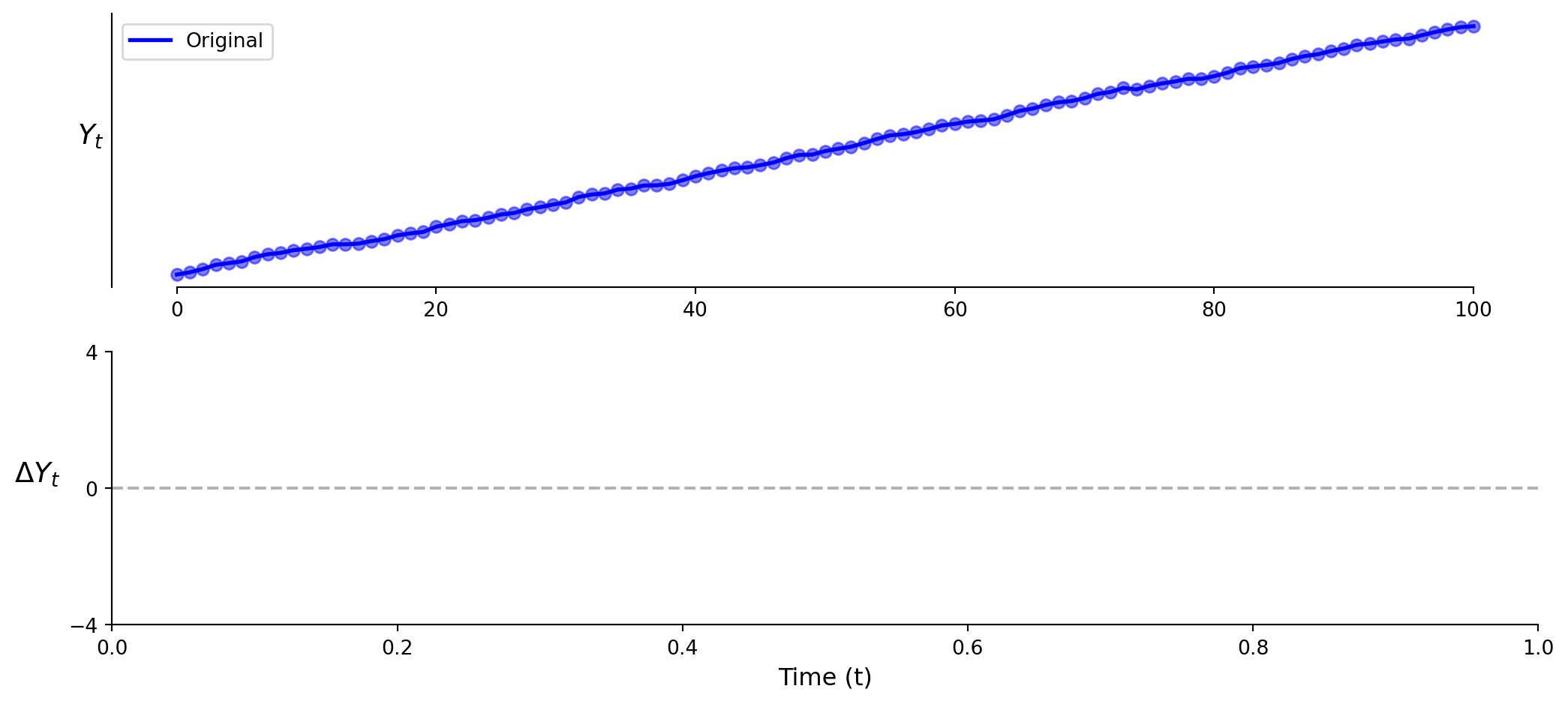
What would first differences look like if there WAS a positive trend?
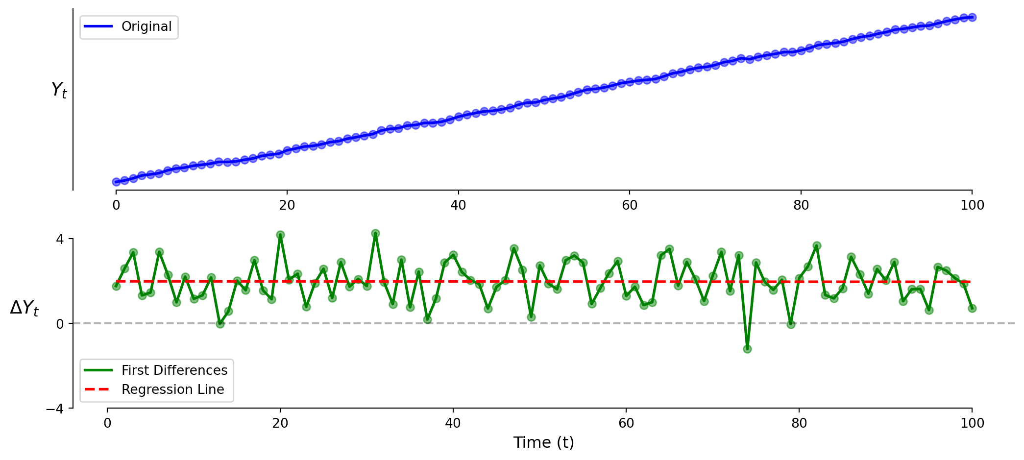
Timeseries: Model 2 (First Differences)
Timeseries: Model 2 (First Differences)
The vertical intercept \(\beta_0\) is positive!
The slope coefficient \(\beta_1\) is zero!
Timeseries: Model 2 (First Differences)
Exercise 4.4 | Model 2
# Step 1. Create first differences of Y 'gdp_diff' ] = data['gdp' ].diff()= data.dropna()
# Step 2. Fit the model (Y differenced, X in levels) = smf.ols('gdp_diff ~ unemployment' , data= data).fit()print (model2.summary().tables[1 ])
# Step 3. Residual and lagged residual plots
Timeseries: Model 3 (Double First Differences)
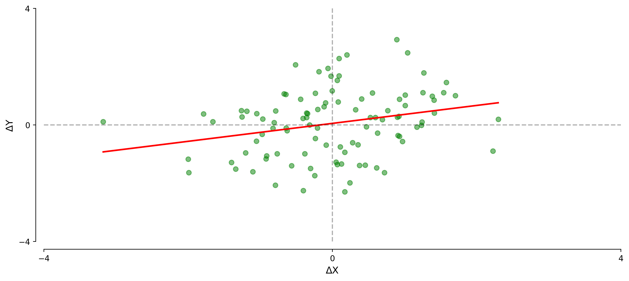
\[\Delta \text{Y}_t = \beta_0 + \beta_1 \times \Delta \text{X}_t + \varepsilon_t\]
Timeseries: Model 3 (Double First Differences)
\[\Delta \text{Y}_t = \beta_0 + \beta_1 \times \Delta \text{X}_t + \varepsilon_t\]
Further reduces serial correlation in the error terms.
\(\beta_0\) captures time trend in \(Y\) \(\beta_1\) captures the short-term relationship between variables.Clear interpretation: how do changes in X relate to changes in Y?
Exercise 4.4 | Model 3
# Step 1. Create first differences of X 'unemployment_diff' ] = data['unemployment' ].diff()= data.dropna()
# Step 2. Fit the double differences model (both X and Y differenced) = smf.ols('gdp_diff ~ unemployment_diff' , data= data).fit()print (model3.summary().tables[1 ])
# Step 3. Residual and lagged residual plots
\(\beta_1\) now represents the short-term relationship between changes in X and Y
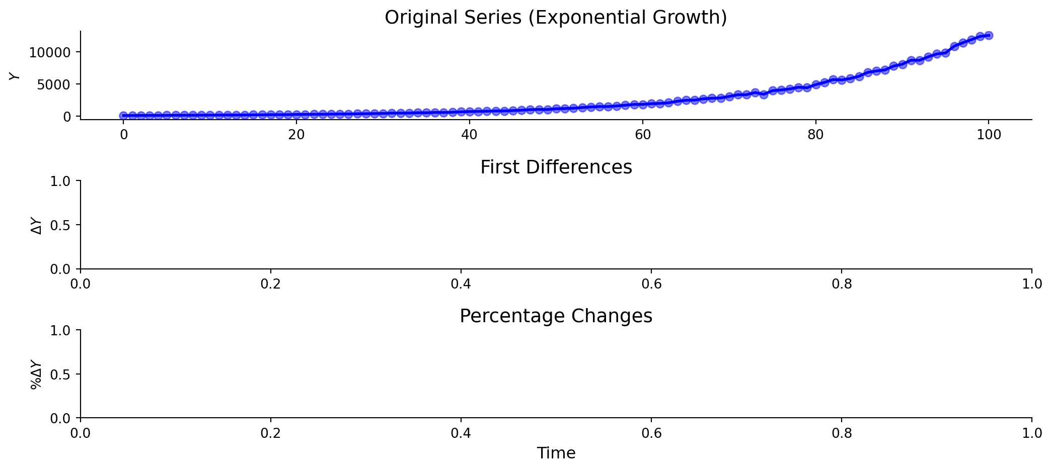
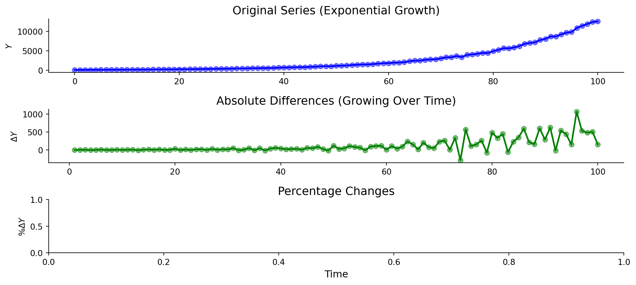
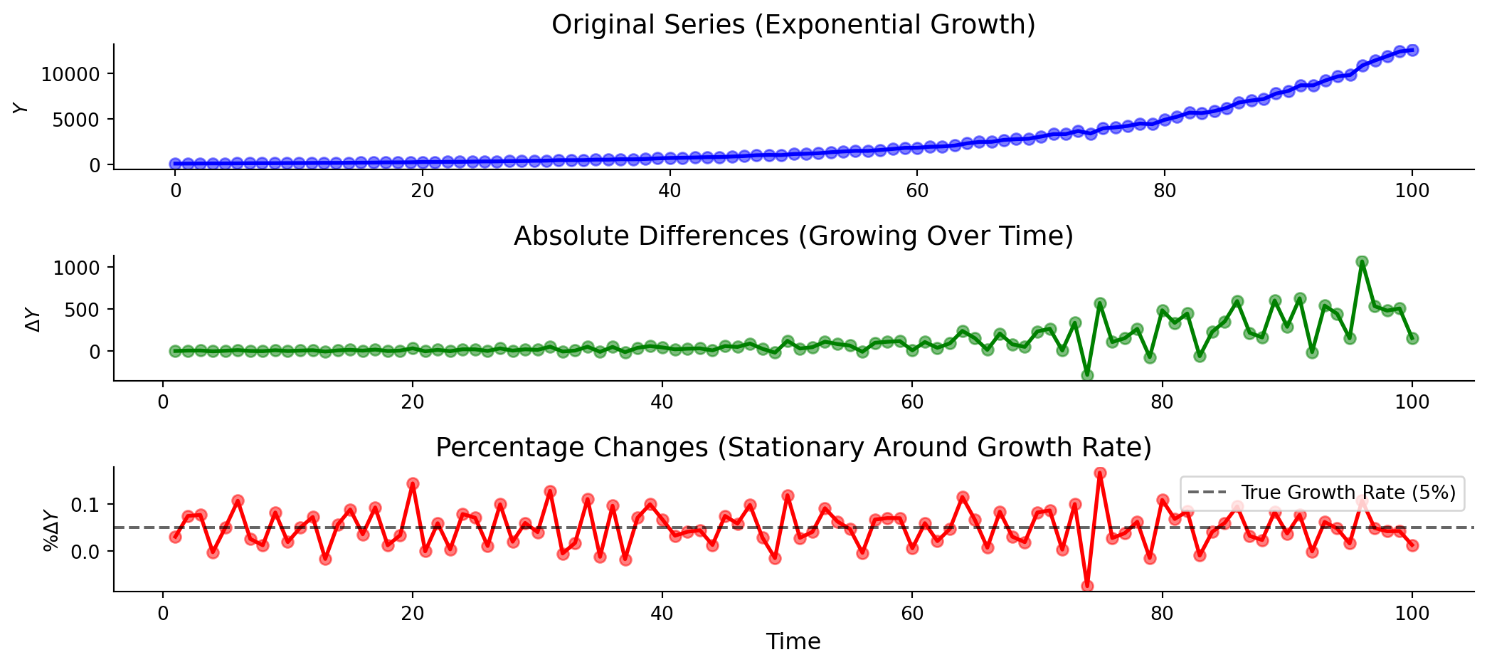
Timeseries: Model 4 (Growth Rates)
\[g_Y = \frac{\text{Y}_t - \text{Y}_{t-1}}{\text{Y}_{t-1}} = \frac{\Delta \text{Y}_t}{\text{Y}_{t-1}}\]
Timeseries: Model 4 (Growth Rates)
\[g_Y = \frac{\text{Y}_t - \text{Y}_{t-1}}{\text{Y}_{t-1}} = \frac{\Delta \text{Y}_t}{\text{Y}_{t-1}}\]
Timeseries: Model 4 (Growth Rates)
\[g_Y = \frac{\text{Y}_t - \text{Y}_{t-1}}{\text{Y}_{t-1}} = \frac{\Delta \text{Y}_t}{\text{Y}_{t-1}}\]
Timeseries: Model 4 (Growth Rates)
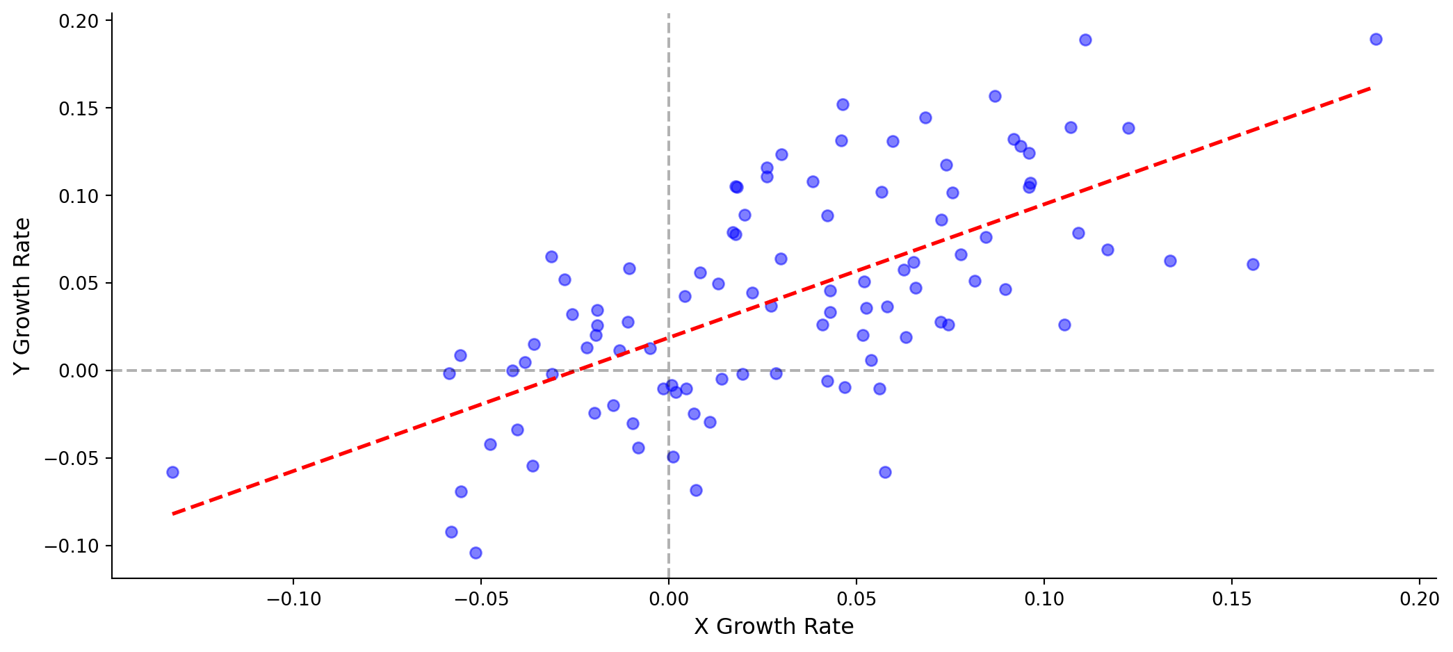
\[g_Y = \beta_0 + \beta_1 \times g_X + \varepsilon_t\]
Timeseries: Model 4 (Growth Rates)
\[g_Y = \beta_0 + \beta_1 \times g_X + \varepsilon_t\]
Growth rate models have the advantages of first differences and can scale better.
This is natural for variables with exponential growth.
\(\beta_0\) is Y’s baseline growth rate.\(\beta_1\) is how Y’s growth responds to a 1 percentage point increase in X’s growth.
Exercise 4.4 | Model 4
# Step 1. Calculate growth rates (percentage changes) 'gdp_growth' ] = data['gdp' ].pct_change() # in percentage points 'unemployment_growth' ] = data['unemployment' ].pct_change()
# Step 2. Drop rows with NaN values = data.dropna()
# Step 3. Fit the growth rate model = smf.ols('gdp_growth ~ unemployment_growth' , data= data).fit()print (model4.summary().tables[1 ])
# Step 4. Residual and lagged residual plots \(\beta_1\) is now expressed in percentage point terms
Timeseries: Summary
Levels
\(Y = \beta_0 + \beta_1 X + \varepsilon\) Relationship between levels
Cross-sectional data
First Diff
\(\Delta Y = \beta_0 + \beta_1 \Delta X + \varepsilon\) Short-term relationship between changes
Trending time series
Growth Rates
\(g_Y = \beta_0 + \beta_1 g_X + \varepsilon\) Response of \(Y\) ’s growth to \(X\) ’s growth
Exponentially growing series
Always check the residual lag plot. Differencing reduces autocorrelation but rarely eliminates it entirely.