ECON 0150 | Economic Data Analysis

The economist’s data analysis skillset.

Part 4.3 | Model Assumptions

GLM (so far)

We’ve built three models. Can we trust them?

1. Each model produces coefficients, standard errors, and p-values.
2. Sometimes a linear model isn’t appropriate.

GLM Assumptions

Which model do you think offers better predictions?

GLM Assumptions

Which model do you think offers better predictions?

Model 1 has predictions close to the average data for all predictor values.

Model 2 will offer inaccurate predictions for large predictor variables!

GLM Assumptions

Our test results are only valid when the model assumptions are valid.

1. Linearity: The relationship between X and Y is linear
2. Homoskedasticity: Equal error variance across all values of X
3. Independence: Observations are independent from each other
4. Normality: Errors are normally distributed

GLM Assumptions: why check?

Assumption violations affect our inferences

If assumptions are violated:

• Coefficient estimates may be biased
• Standard errors may be wrong
• p-values may be misleading
• Predictions may be unreliable

We use residuals (\(\epsilon\)) and estimates (\(\hat{y}\)) to check if a model is ‘specified’.

Model Fit

We use residuals (\(\varepsilon\)) and estimates (\(\hat{y}\)) to check if a model is ‘specified’.

Residuals (\(\varepsilon\)): the error of each prediction; how far off the model is.

Estimates (\(\hat{y}\)): the model’s predicted value for each observation.

Exercise 4.3 | Happiness and GDP

Use a residual plot to visualize the error for the model.

# Calculate residuals and predictions
residuals = model.resid
predictions = model.predict()

# Residual Plot: predictions against residuals
plt.scatter(predictions, residuals)

Assumption 1: Linearity

The error term should be unrelated to the fitted value.

Q. Which model appears to violate the Linearity Assumption?

Assumption 1: Linearity

The error term should be unrelated to the fitted value.

Q. Which model appears to violate the Linearity Assumption?

Model 1 is equally wrong everywhere. Model 2 has larger errors at the extremes.

Assumption 1: Linearity

A non-linear relationship will produce non-linear residuals.

The linear model misses the true curvature leading to systematic errors.

Handling Non-Linear Relationships

Transform variables to become linear

Adding a square term or performing a log transformation can fix the problem.

instead of

\[\text{income} = \beta_0 + \beta_1 \text{age} + \varepsilon\]

we could use

\[\text{income} = \beta_0 + \beta_1 \text{age} + \beta_2 \text{age}^2 + \varepsilon\]

It’s also common to log transform either the \(x\) or \(y\) variable.

Assumption 2: Homoskedasticity

Residuals should be spread out the same everywhere.

Q. Which one of these figures shows homoskedasticity?

Assumption 2: Homoskedasticity

Residuals should be spread out the same everywhere.

Q. Which one of these figures shows homoskedasticity?

Model 1 is equally wrong everywhere. Model 2 has errors that grow with the fitted value.

Assumption 2: Homoskedasticity

The spread of residuals should not change across values of X.

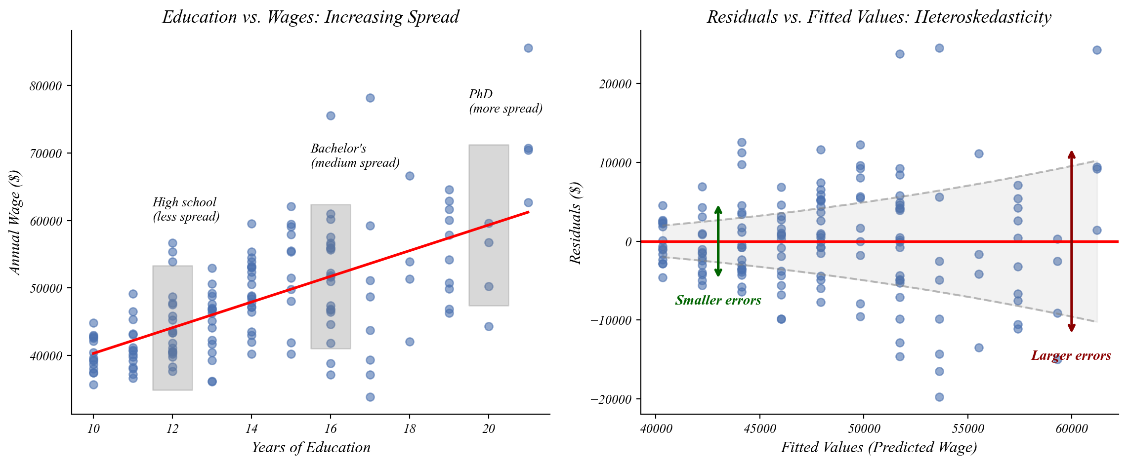
The spread of points increases as education increases!

Handling Heteroskedasticity

Robust standard errors give more accurate measures of uncertainty

Use Robust Standard Errors which adjust for the changing spread, giving more accurate p-values.

# Fit the model with robust standard errors (HC3: heteroskedastic-constant)
robust_model = smf.ols('wages ~ education', data=df).fit(cov_type='HC3')

Assumption 3: Independence

Each error should be unrelated to previous errors.

Q. Which of these residual lag plots shows independence?

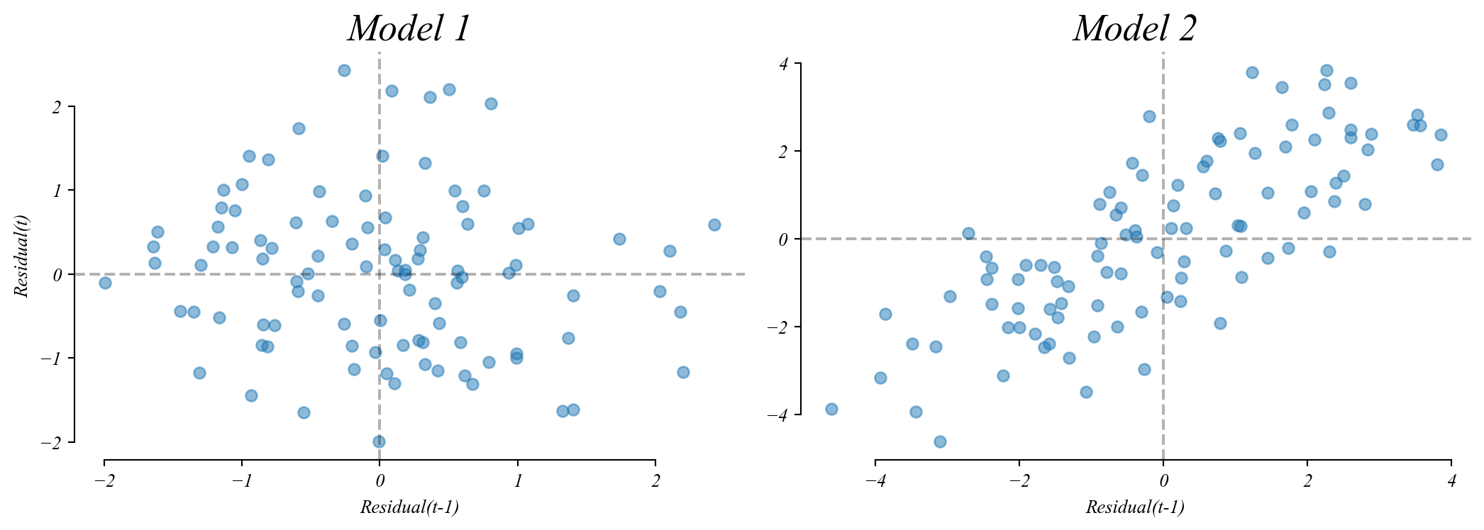
Assumption 3: Independence

Each error should be unrelated to previous errors.

Q. Which of these residual lag plots shows independence?

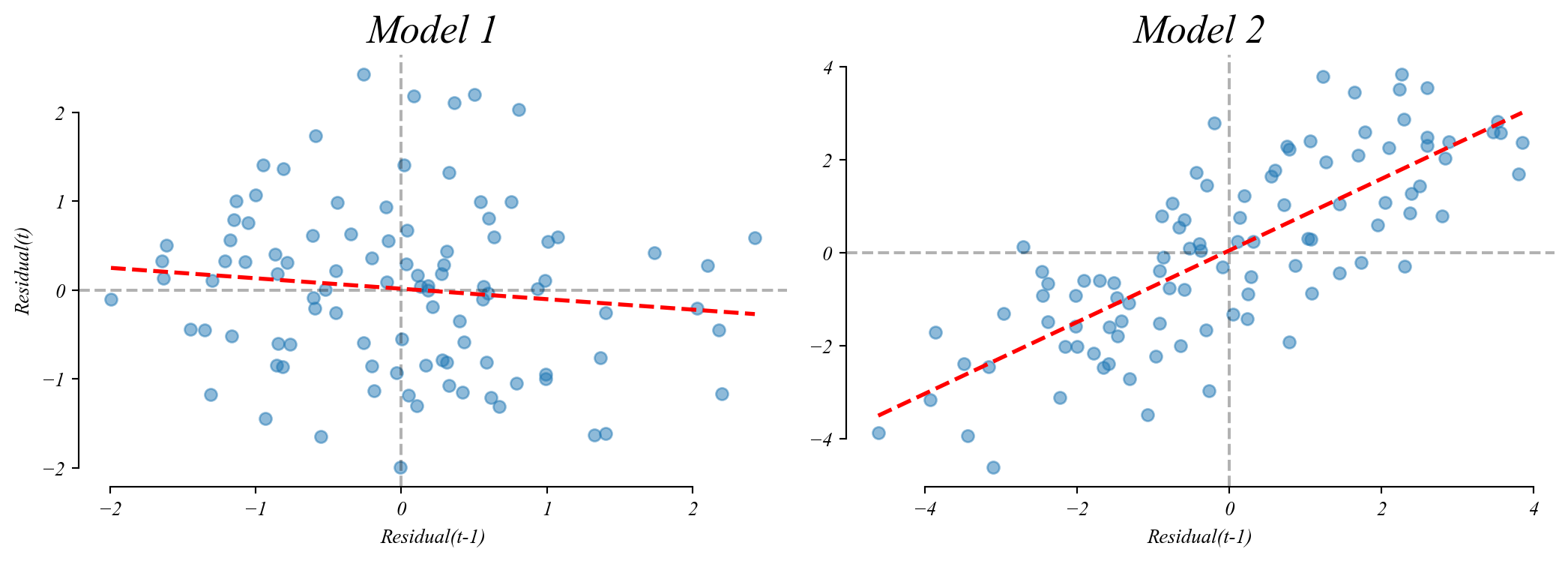
Model 1 has no (meaningful) relationship between consecutive residuals.

Model 2 shows a positive relationship (autocorrelation).

Checking Independence

Use a lagged residual plot to check for autocorrelation.

# Create lagged residuals
lagged_residuals = residuals[:-1]
current_residuals = residuals[1:]

# Lag plot
plt.scatter(lagged_residuals, current_residuals)

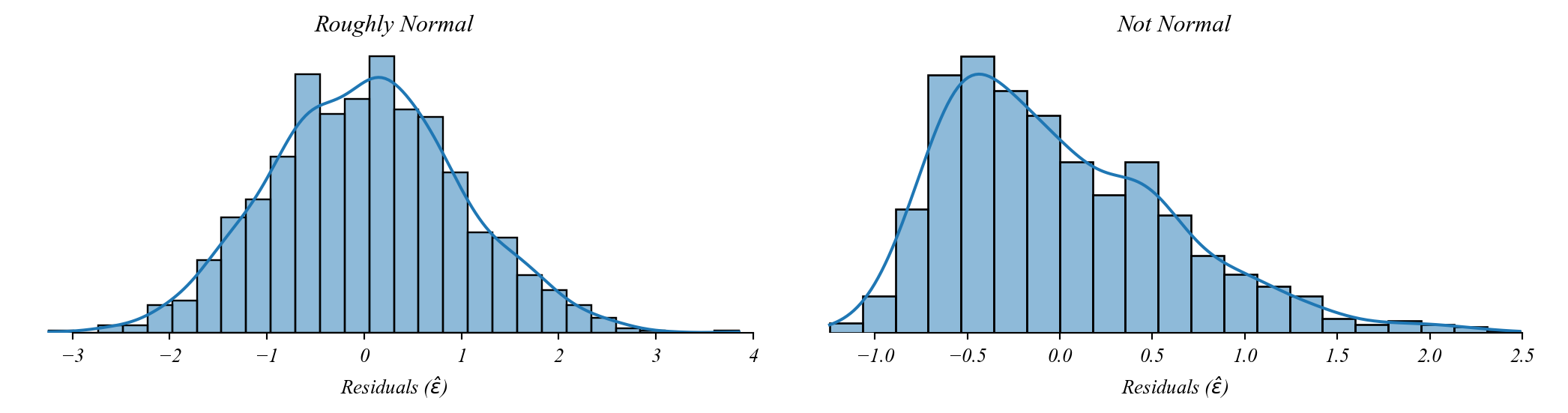
Assumption 4: Normality

Residuals should be normally distributed.

By the CLT we can still use GLM without this so long as the sample is large.

Looking Forward

Extending the GLM framework

Next Up:

• Part 4.4 | The Problem of Timeseries

Later:

• Part 5.1 | Numerical Controls
• Part 5.2 | Categorical Controls
• Part 5.3 | Interactions
• Part 5.4 | Model Selection

> all built on the same statistical foundation