ECON 0150 | Economic Data Analysis

The economist’s data analysis workflow.

Part 4.2 | Categorical Predictors

GLM: The story so far

We’ve built two models. Now we need a third.

Q. Do neighborhoods with greenspace have lower temperatures?

We need a new approach, but we already have the tools.

GLM: City Greenspace and Temperature

Q. Is temperature lower in neighborhoods with more green space?

What is the variable type of High Greenspace?

Q. Does temperature change as we increase by one on the horizontal axis?

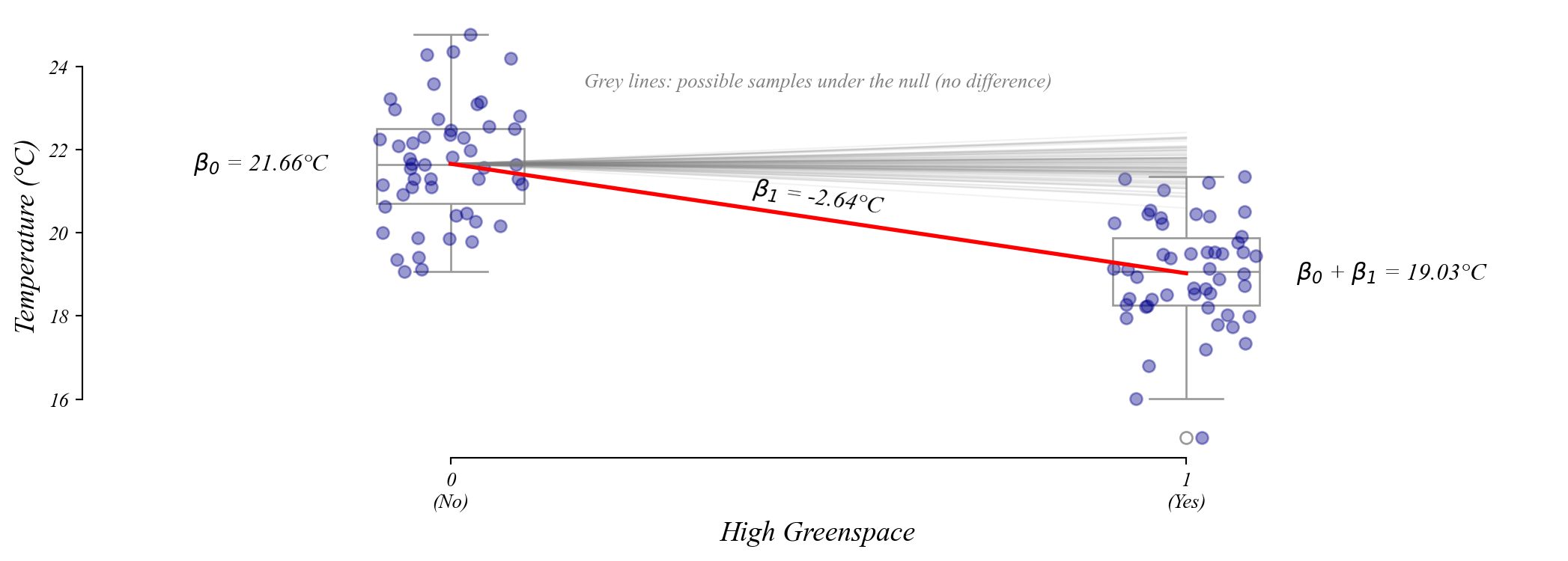
\[Temperature = \beta_0 + \beta_1 \cdot HighGreen + \varepsilon\]

GLM: City Greenspace and Temperature

Q. Is temperature lower in neighborhoods with more green space?

1. The GLM framework doesn’t care whether \(x\) is continuous or binary. We code the group as 0 and 1, and fit the same model.

2. Like with numerical predictors, the GLM tests whether \(\beta_1\) is different from zero.

GLM: City Greenspace and Temperature

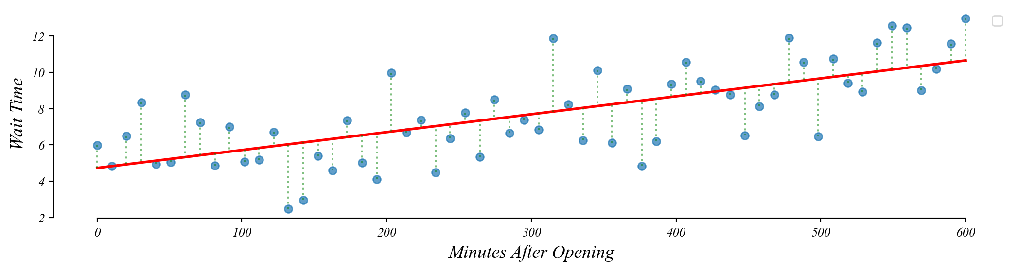
Q. Does temperature change as we move out on the horizontal axis?

\[Temperature = \beta_0 + \beta_1 \cdot HighGreen + \varepsilon\]

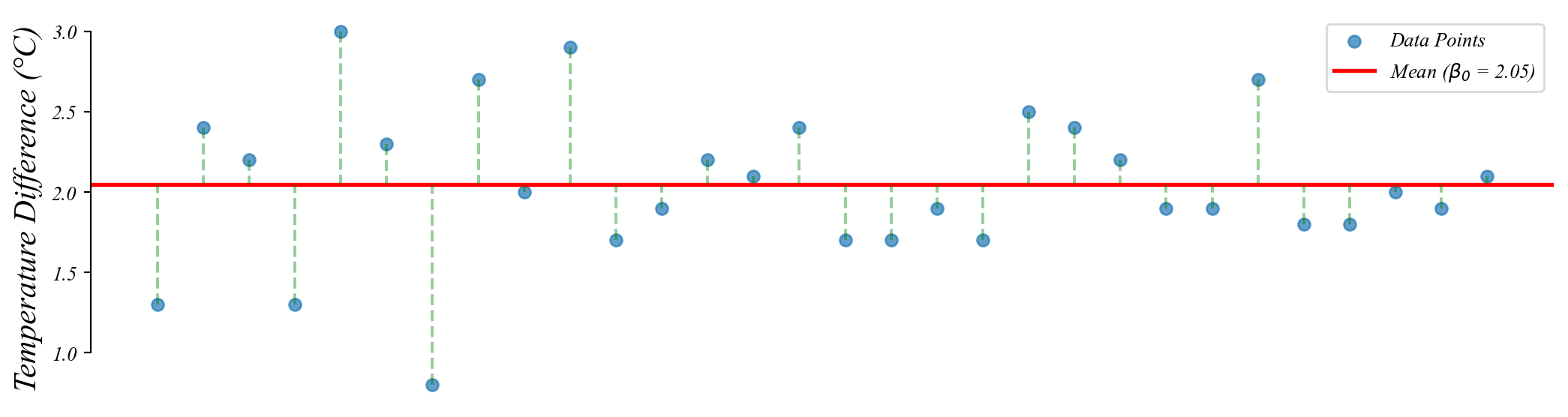
How would we interpret \(\beta_0\) here?

> \(\beta_0\) is the mean temperature in (\(x=0\)) low green space cities (22.03°C)

GLM: City Greenspace and Temperature

Q. Does temperature change as we move out on the horizontal axis?

\[Temperature = \beta_0 + \beta_1 \cdot HighGreen + \varepsilon\]

How would we interpret \(\beta_1\) here?

> Cities with Green Space (x=1) have a temperature that is lower by \(\beta_1\)

> ie. a one unit increase in \(x\) changes temperature by \(\beta_1\)

Categorical GLM: sampling error

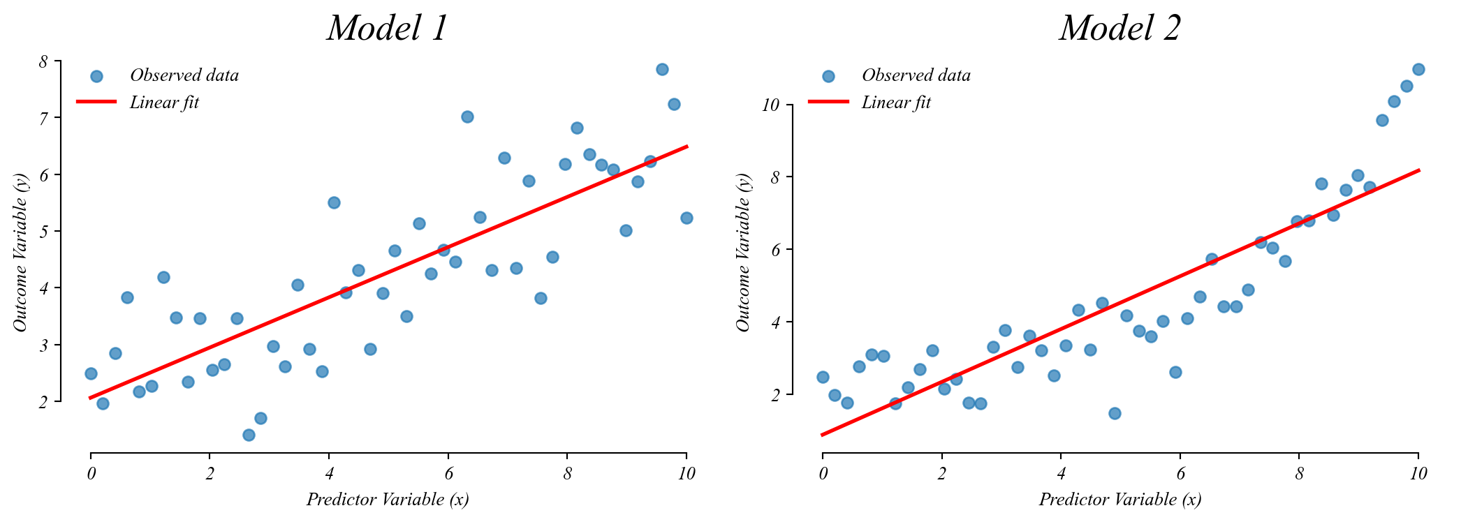
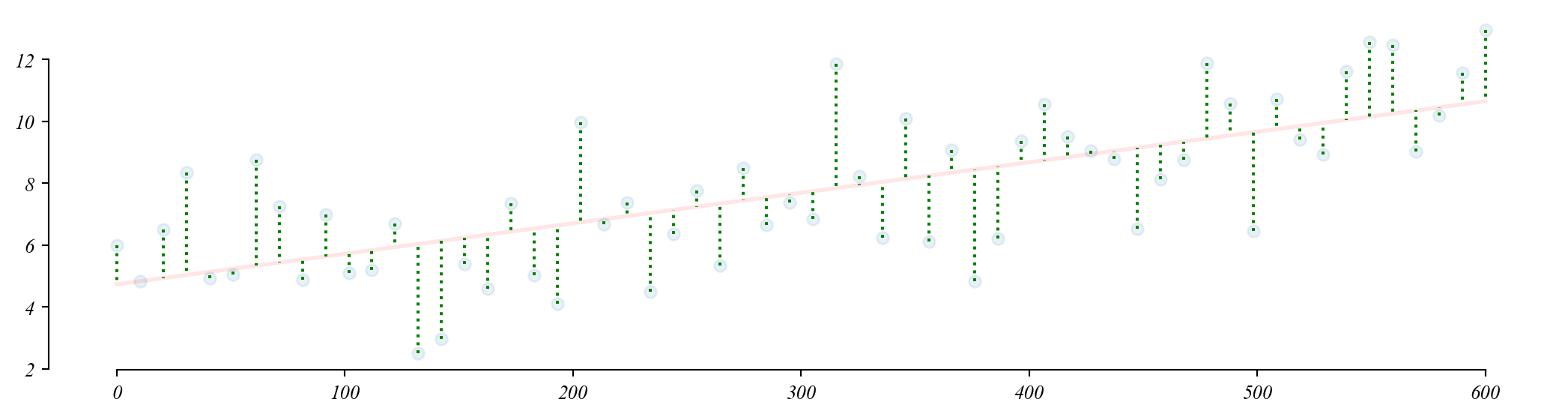
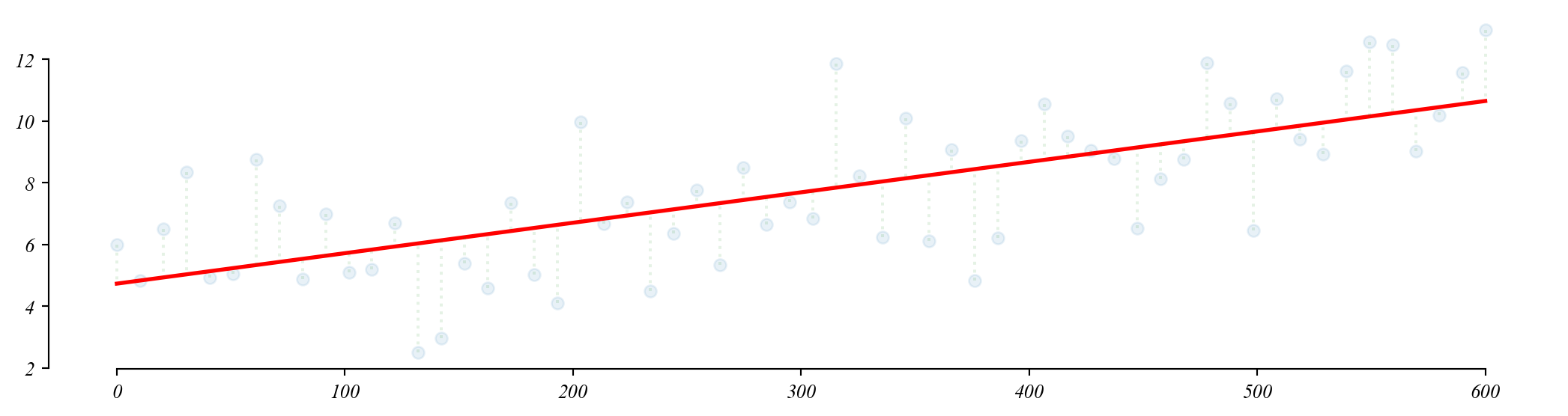
Like before, if we take many samples, we get slightly different slopes and slightly different fits.

Categorical GLM: sampling distribution of slopes

The slope coefficient follows a normal distribution centered on the population difference.

> the slopes follow a normal distribution around the population difference!

> this lets us perform a t-test on the slope!

Categorical GLM: sampling distribution of slopes

The slope coefficient follows a normal distribution centered on the population difference.

> we don’t know the entire distribution, just our sample slope

Categorical GLM: sampling distribution of slopes

The slope coefficient follows a normal distribution centered on the population difference.

> center the distribution on our null

> check the distance from the sample

Categorical GLM: sampling distribution of slopes

The slope coefficient follows a normal distribution centered on the population difference.

> p-value: the ‘surprisingness’ of our sample if \(\beta_1 = 0\)

> the probability of seeing our sample by chance if there is no difference

> a small p-value is evidence against the null hypothesis (\(\beta_1 = 0\))

Categorical GLM: null slopes

Many possible slopes we might observe by chance if the null (\(\beta_1 = 0\)) were true.

> how likely does it look like this slope was drawn from the null slopes?

> p-value: the probability of a slope as extreme as ours under the null (\(\beta_1=0\))

This is a two-sample t-test

This is a simpler view of a t-test.

1. Estimating differences between group means is exactly a two-sample t-test.

2. GLM is a general framework that can handle in one modeling approach:

• Numerical predictors
• Categorical predictors
• Control variables (later)

3. The two-sample t-test is a special case of the GLM.

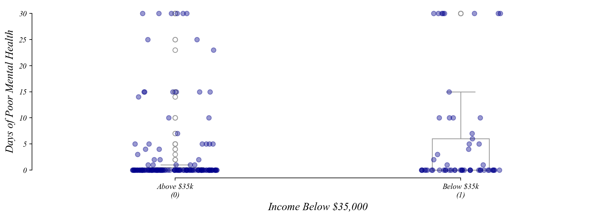
Exercise: Income and Mental Health

Do individuals earning under $35,000 report more poor mental health days?

Step 1: Summarize the data

# Load BRFSS data
data = pd.read_csv('data/BRFSS_cleaned.csv')
data['low_income'] = (data['INCOME2'] <= 5).astype(int)

# Visualize Binary Predictor
sns.boxplot(data=data, x='low_income', y='MENTHLTH', color='white', width=0.2)
plt.xticks([0,1], labels=['Above $35k', 'Below $35k']  # INCOME2 <= 5)

Exercise: Income and Mental Health

Do individuals earning under $35,000 report more poor mental health days?

Step 2: Build a model

\[MentalHealthDays = \beta_0 + \beta_1 \cdot LowIncome + \varepsilon\]

Exercise: Income and Mental Health

Do individuals earning under $35,000 report more poor mental health days?

Step 3: Estimate the model

# Model: y = b + mx
model = smf.ols('MENTHLTH ~ low_income', data).fit() # Intercept is included by default
print(model.summary().tables[1])

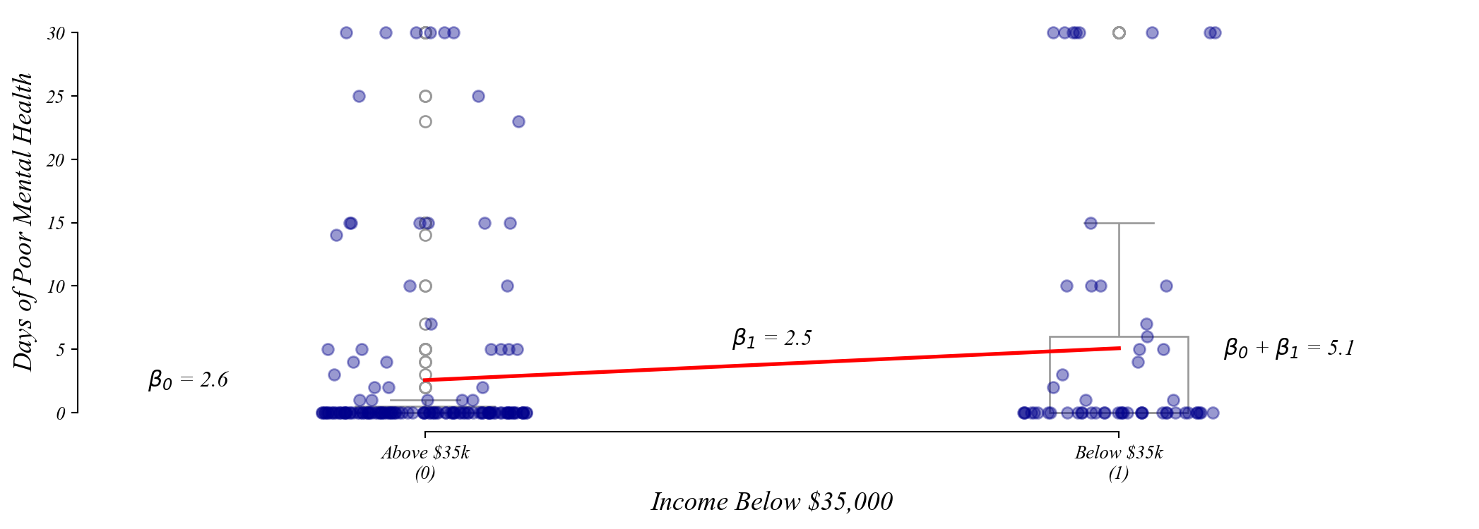
• \(\beta_0\) = Mean poor mental health days for those earning above $35k

• \(\beta_1\) = Additional poor mental health days for those earning below $35k

Exercise: Income and Mental Health

Do individuals earning under $35,000 report more poor mental health days?

Step 4: Check the residuals (next time)

sns.scatterplot(x=model.predict(), y=model.resid, alpha=0.5)
plt.axhline(y=0, color='red', linestyle='-')
plt.xlabel('Fitted Values')
plt.ylabel('Residuals')

> what do you notice about this residual plot?

Exercise: Income and Mental Health

Do individuals earning under $35,000 report more poor mental health days?

Step 5: Interpret and communicate the findings

> A significant positive \(\beta_1\) suggests those earning under $35k report more poor mental health days per month

> but does low income cause poor mental health, or are other factors at play?

The General Linear Model (so far)

Extending the GLM framework

• Part 3 | Intercept-Only Model | \(y = \beta_0 + \epsilon\)

• Part 4.1 | Numerical Predictor | \(y = \beta_0 + \beta_1 x + \epsilon\)

• Part 4.2 | Categorical Predictor | \(y = \beta_0 + \beta_1 x + \epsilon\)

• Part 4.3 | Model Diagnostics

• Part 4.4 | Causality

Looking Forward

Extending the GLM framework

Part 5 | Control Variables

\[y = \beta_0 + \beta_1 x_1 + \beta_2 x_2 + ... + \varepsilon\]

• Part 5.1 | Numerical Controls
• Part 5.2 | Categorical Controls
• Part 5.3 | Interactions
• Part 5.4 | Model Selection

> all built on the same statistical foundation