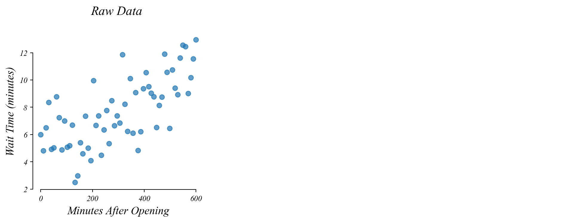
GLM: bivariate data
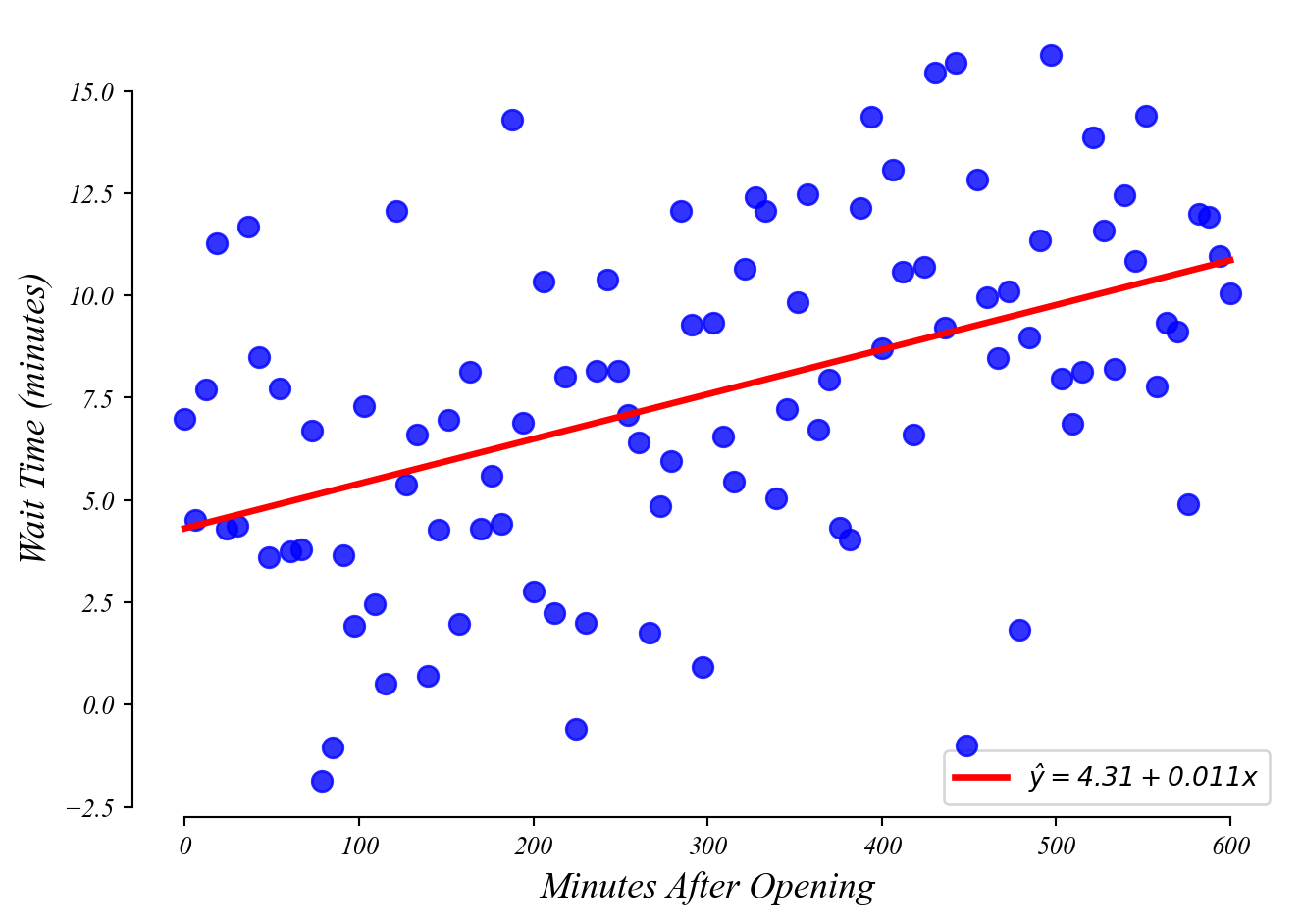
Do people wait longer later in the day?
> but in general we don’t ask many questions about vertical incercepts
GLM: bivariate data
Do people wait longer later in the day?

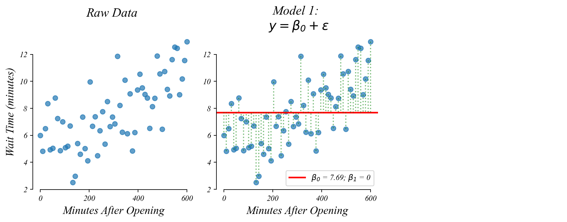
Lets compare two models.
- Model 1 (Intercept Only): \(y = b\)
- Model 2 (Intercept+Slope): \(y = mx + b\)
GLM: bivariate data
Do people wait longer later in the day?
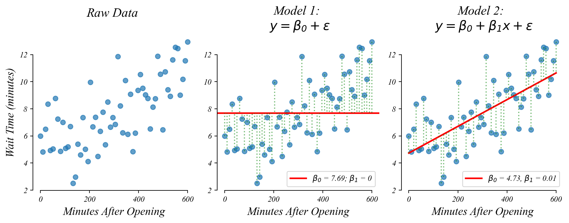
> a slope (β₁) improves model fit (MSE; ‘wrongness’) when there’s a relationship
> the intercept is no longer the mean
Bivariate GLM: minimizing MSE
Which model minimizes the models’ ‘wrongness’ (Mean Squared Error)?
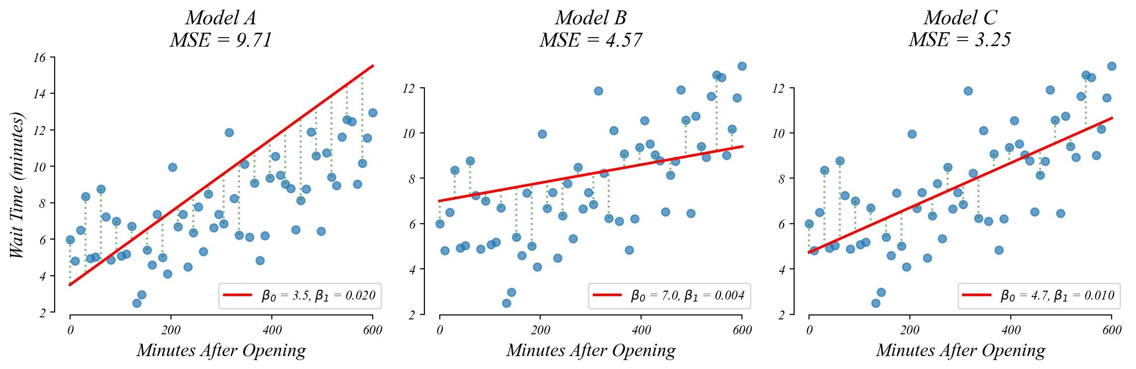
> Model C minimizes MSE!
Bivariate GLM: minimizing MSE
GLM selects the \(\beta_1\) with the smallest MSE.
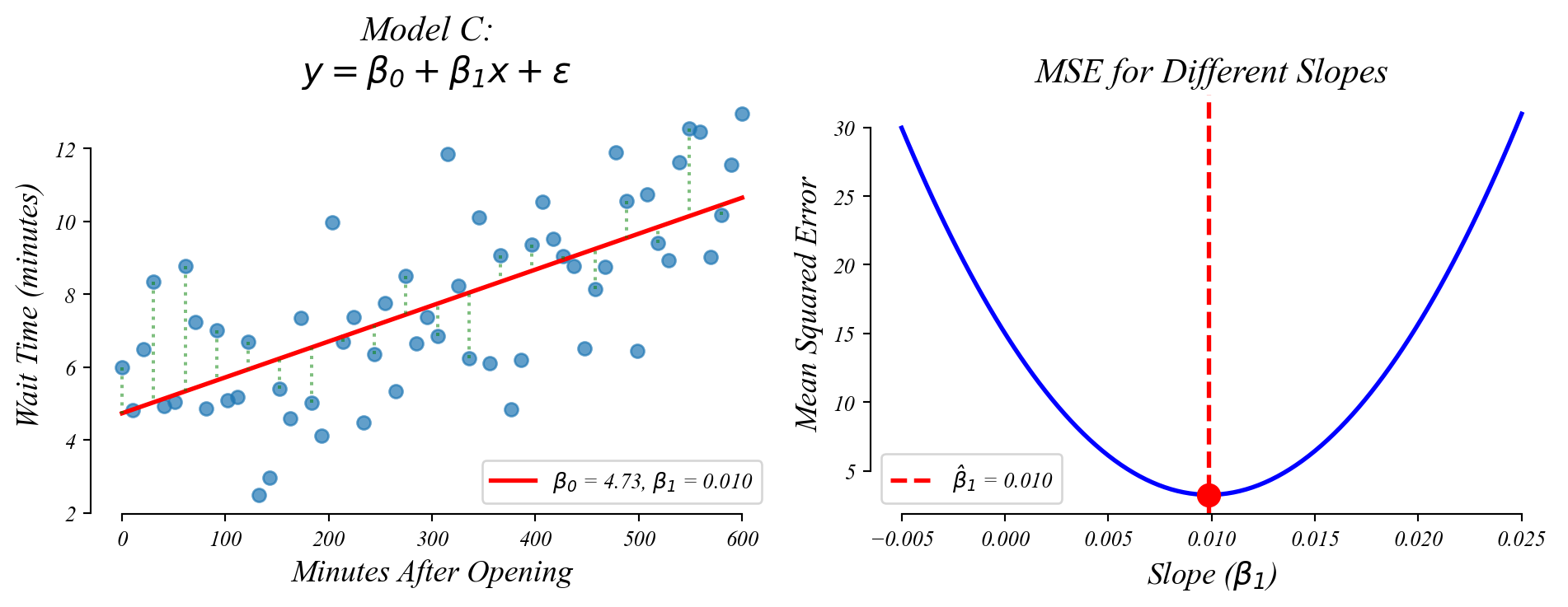
> this slope (β₁) gives the best guess of the relationship between x and y
> but what if the true slope is zero … could this slope be just sampling error?
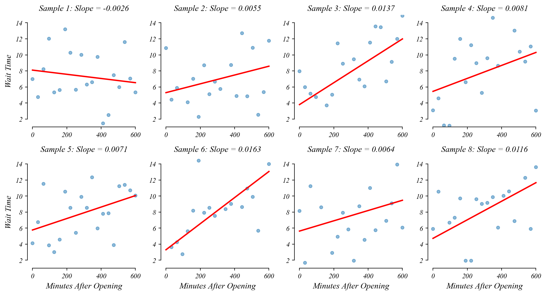
Bivariate GLM: sampling error
Like before, if we take many samples, we get slighly different slopes and slighly different fits.
Bivariate GLM: sampling distribution of slopes
The slope coefficient follows a normal distribution centered on the population slope.
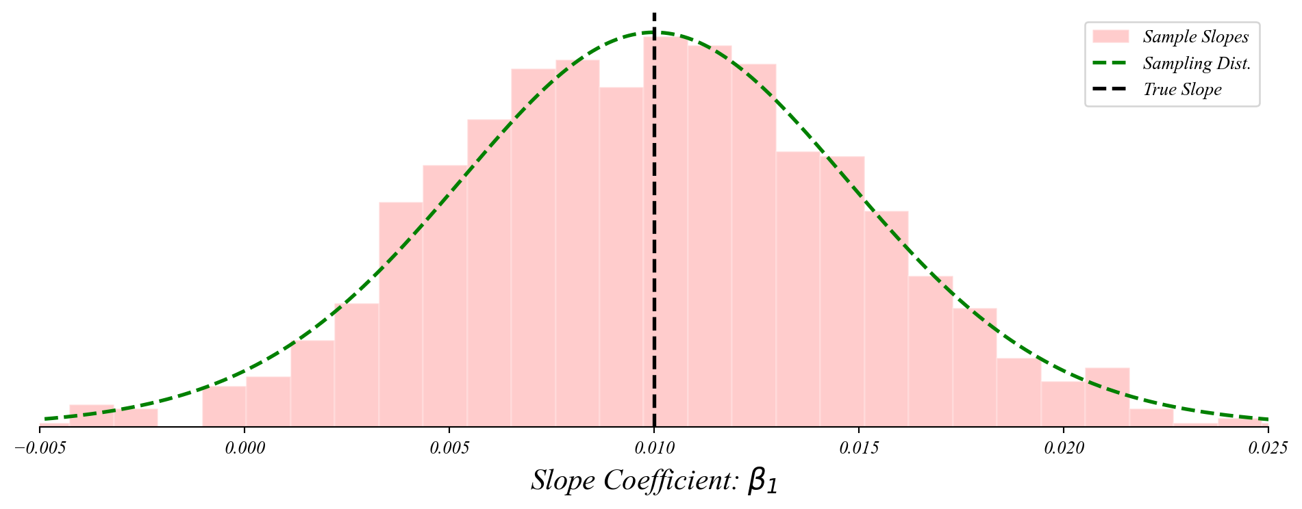
> the slopes follow a normal distribution around the population relationship!
> this lets us perform a t-test on the slope!
Bivariate GLM: sampling distribution of slopes
The slope coefficient follows a normal distribution centered on the population slope.
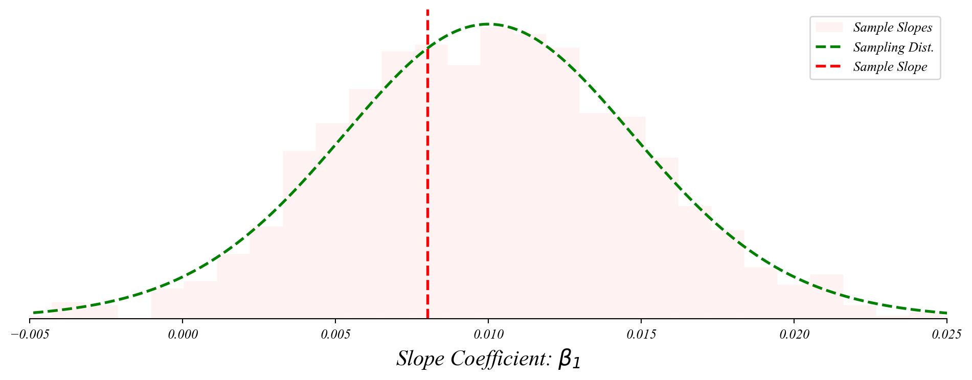
> we don’t know the entire distribution, just our sample slope
Bivariate GLM: sampling distribution of slopes
The slope coefficient follows a normal distribution centered on the population slope.
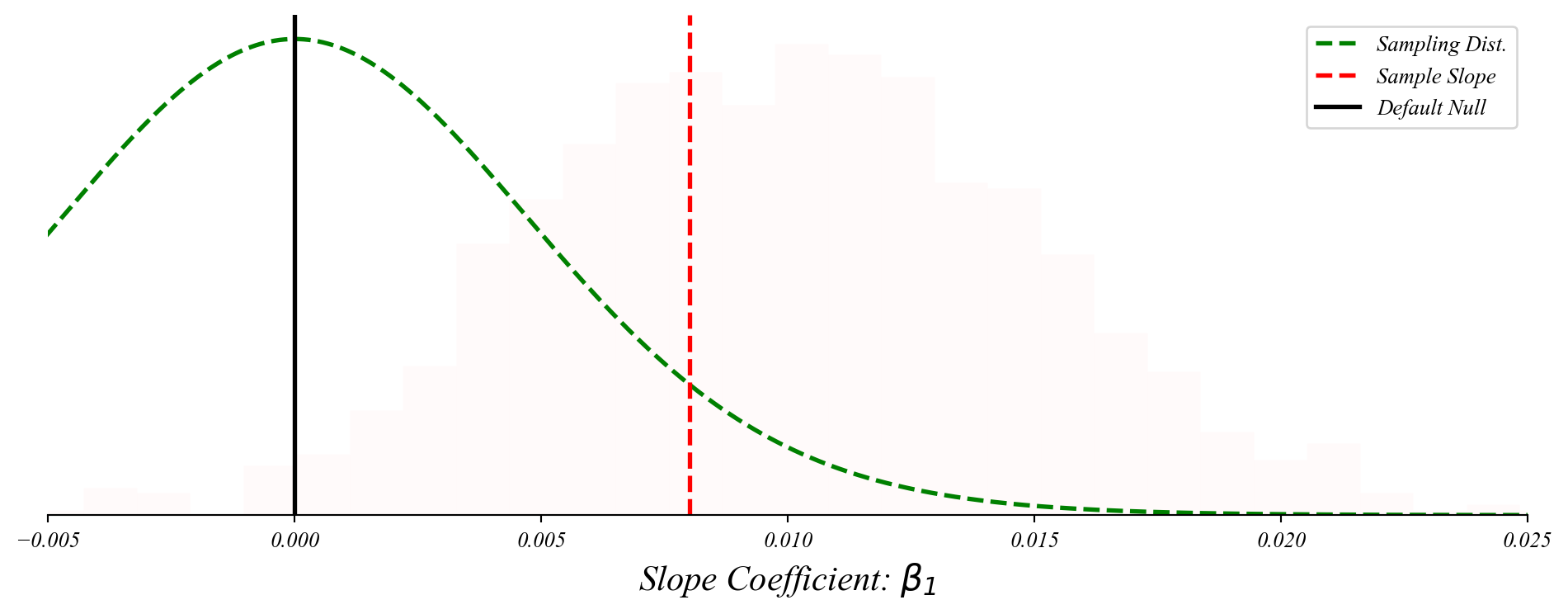
> center the distribution on our null
> check the distance from the sample
Bivariate GLM: sampling distribution of slopes
The slope coefficient follows a normal distribution centered on the population slope.
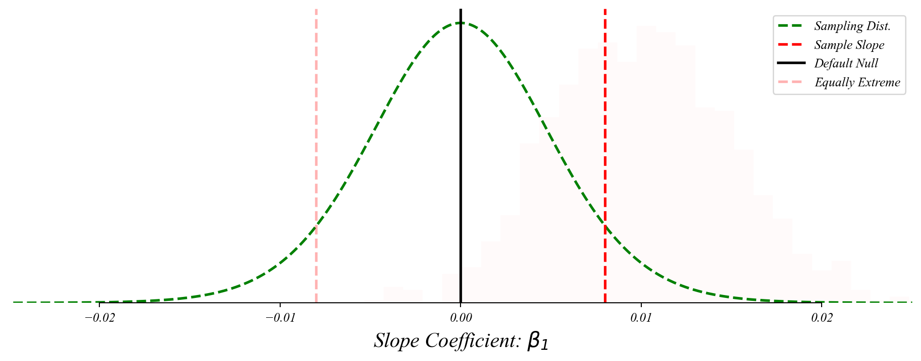
> the p-value is the probability of something as far from the null as our sample
Bivariate GLM: sampling distribution of slopes
The slope coefficient follows a normal distribution centered on the population slope.
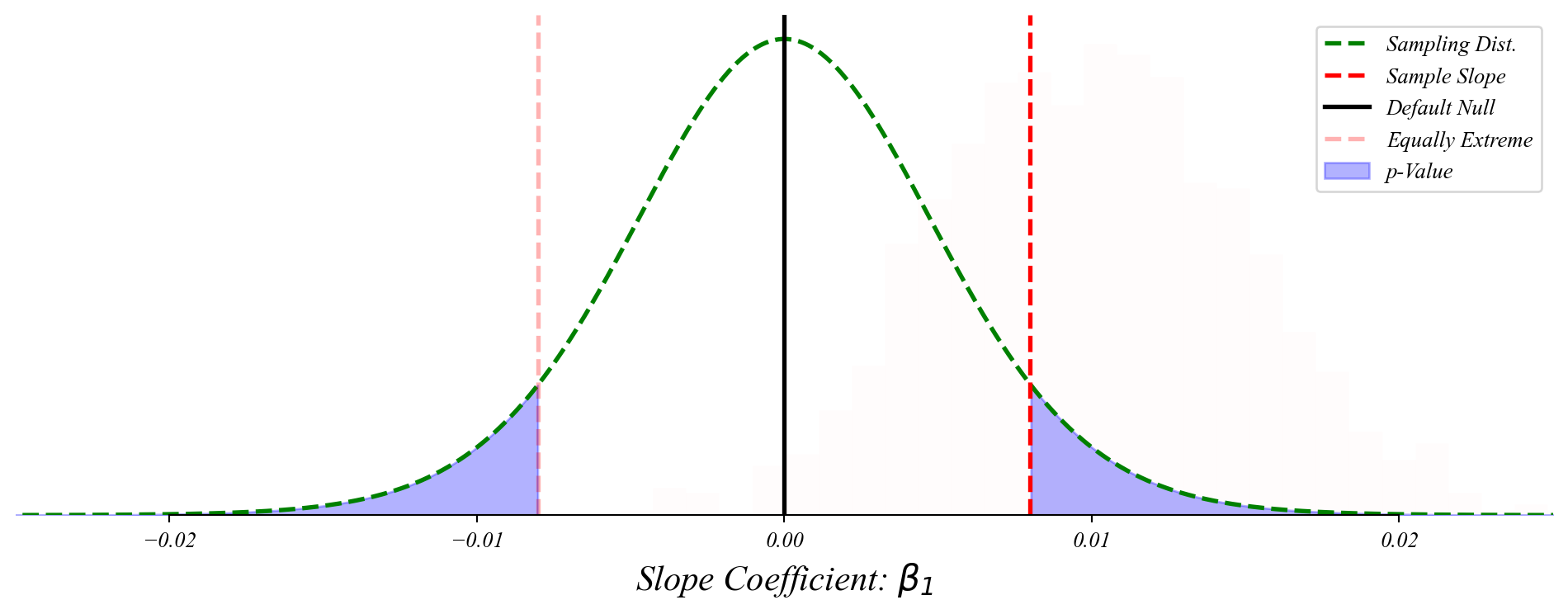
> p-value: the ‘surprisingness’ of our sample if \(\beta_1 = 0\)
> the probability of seeing our sample by chance if there is no relationship
> a small p-value is evidence against the null hypothesis (\(\beta_1 = 0\))
Bivariate GLM: sampling distribution of slopes
Many possible models we might observe by chance if the null (\(\beta_1 = 0\)) were true.
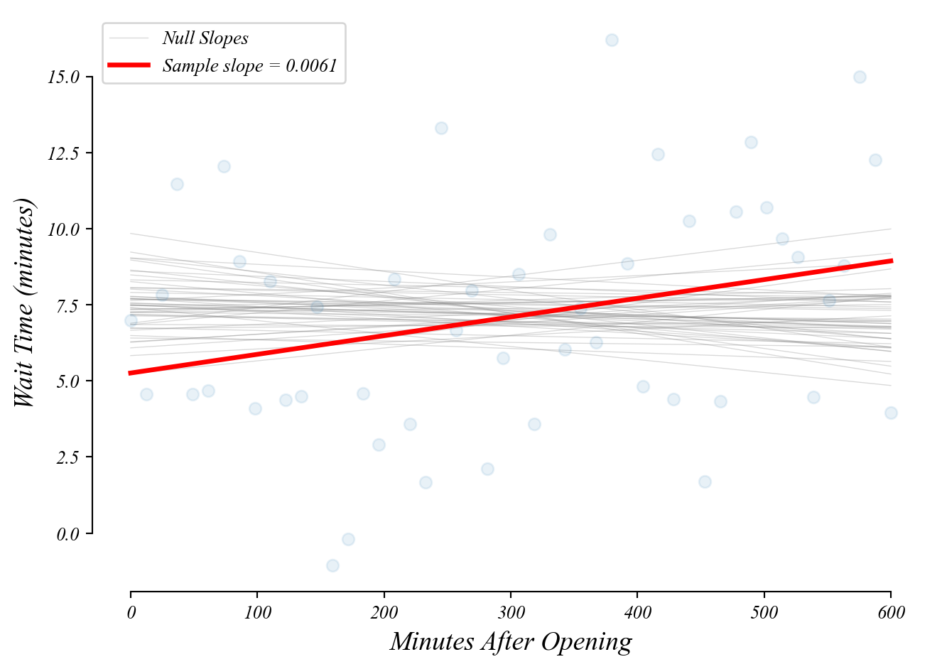
> how likely does it look like this slope was drawn from the null slopes?
> p-value: the probability a slope as extreme as ours under the null (\(\beta_1=0\))
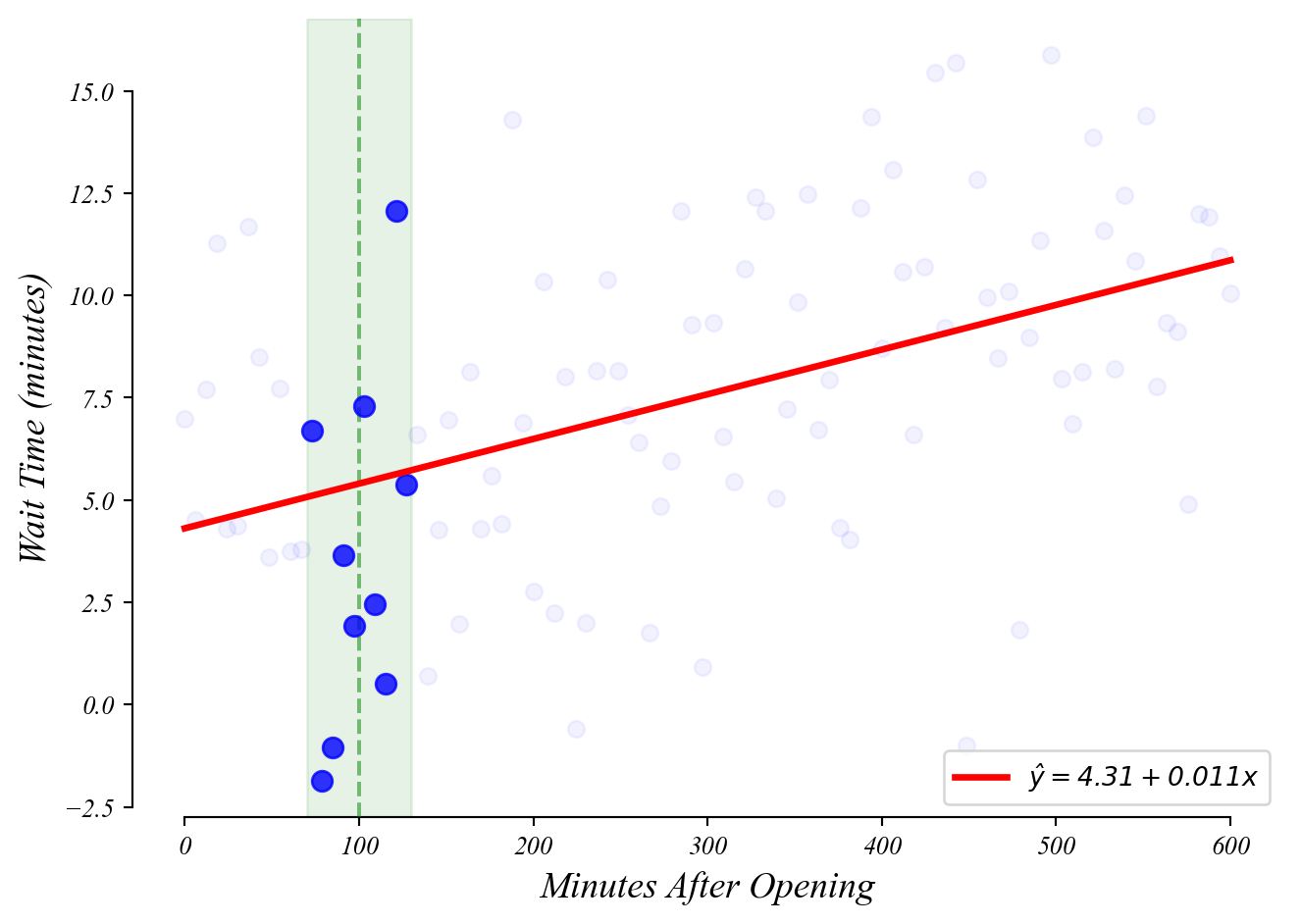
GLM: predictions
What wait time should we expect at 100 minutes after open?
GLM: predictions
What wait time should we expect at 100 minutes after open?
GLM: predictions
What wait time should we expect at 100 minutes after open?
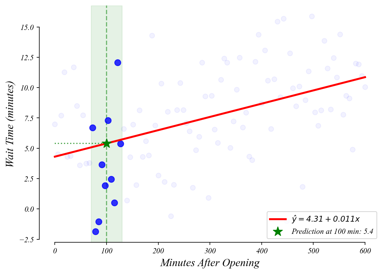
> you can find this with a calculator!
> plug \(x=100\) into the equation \(y = 4.31 + 0.011 x\)
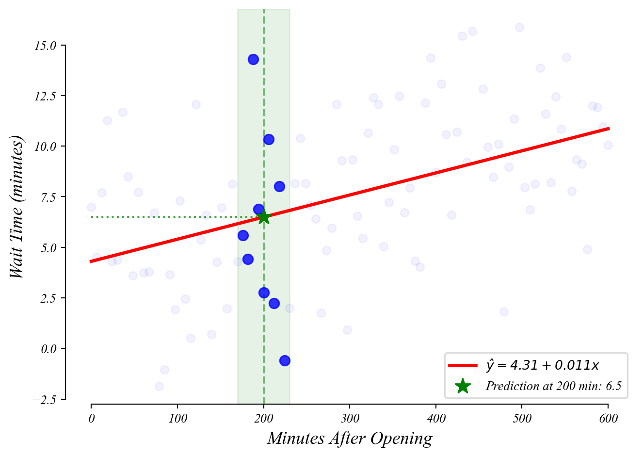
GLM: predictions
What wait time should we expect at 200 minutes after open?
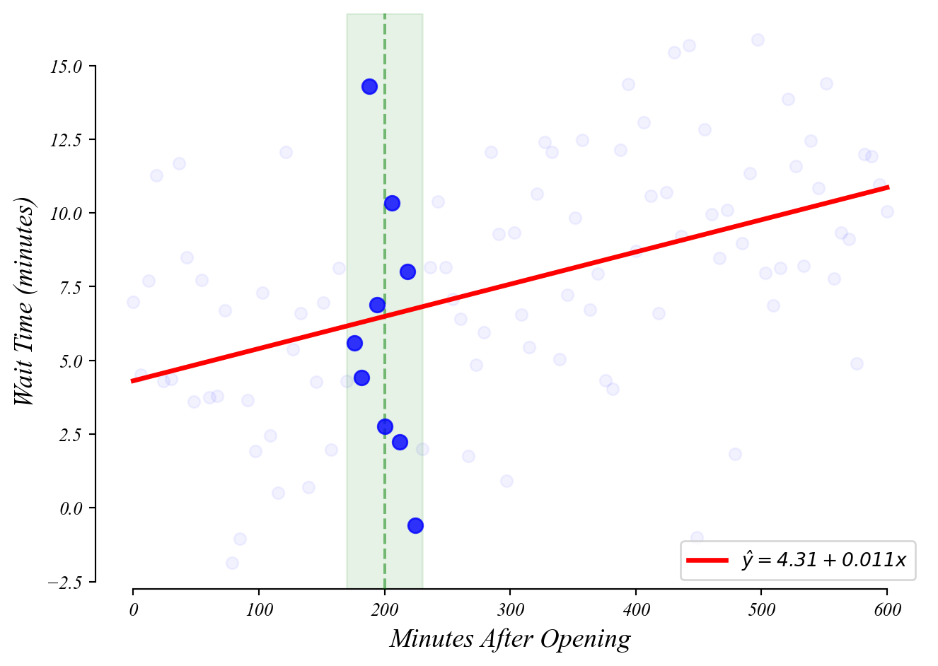
GLM: predictions
What wait time should we expect at 200 minutes after open?
GLM: interpretation
How much does wait time increase every minute after open?
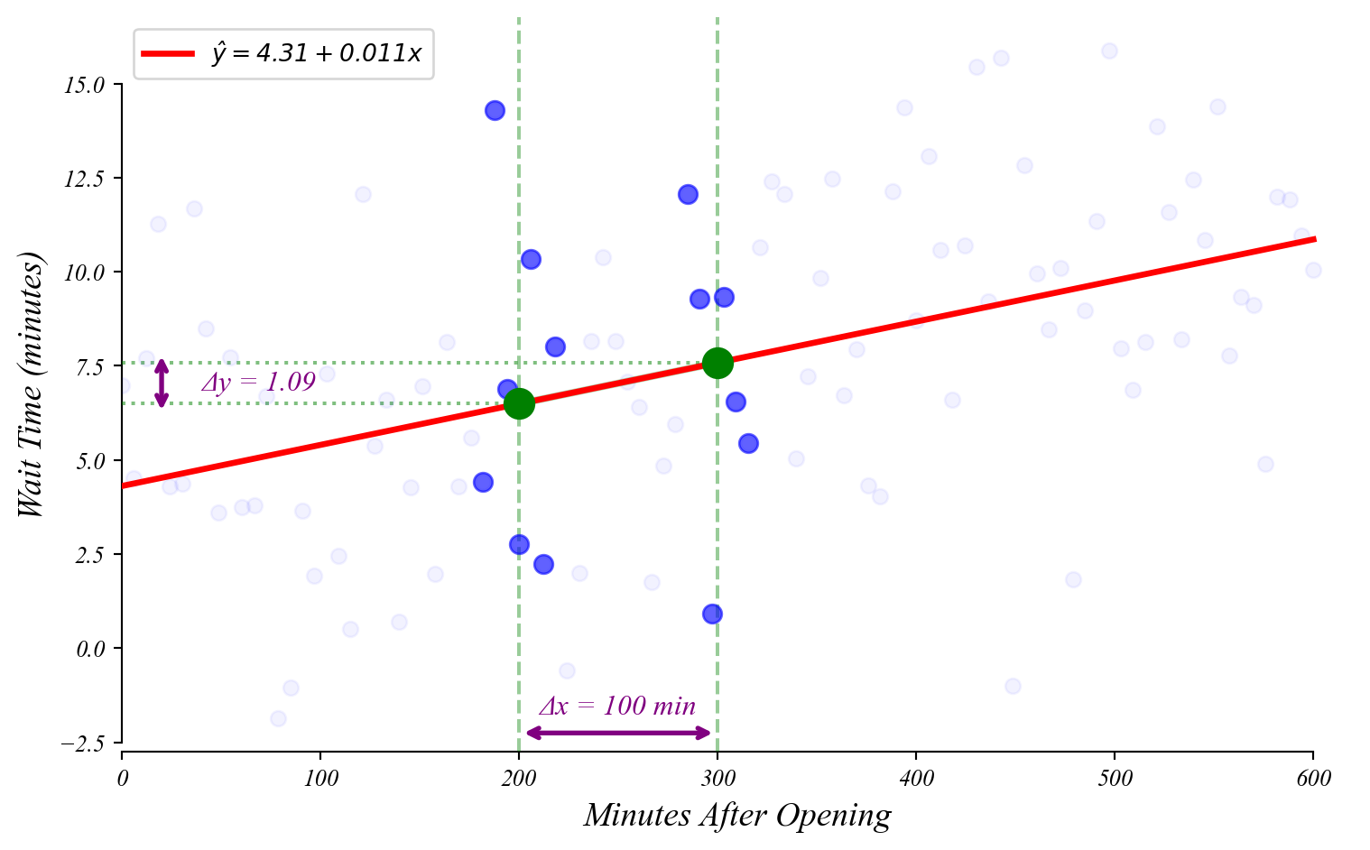
> \(\beta_1\) tells us how much \(y\) increases with every 1 unit increase in \(x\)