ECON 0150 | Economic Data Analysis

The economist’s data analysis skillset.

Part 3.4 | Hypothesis Testing

A Big Question

How do we learn about the population when we don’t know \(\mu\) or \(\sigma\)?

• Part 3.1 | Known Random Variables
  • If we know the random variable, we can answer all kinds of probability questions
• Part 3.2 | Sampling and Unknown Random Variables
  • The sample means of unknown random variables will approximate a normal distribution around the truth
• Part 3.3 | Confidence Intervals
  • We can use the sampling distribution to know the probability that the sample mean (\(\bar{x}\)) will be close to the population mean (\(\mu\))

Sampling Distribution: Unknown \(\mu\); Known \(\sigma\)

If we know the population mean, we know the sampling distribution is approximately normal.

• The sample mean is drawn from an approximately normal distribution with mean \(\mu\) and standard error \(\sigma / \sqrt{n}\).
• Each time we draw a sample we see a different sample mean.
• What do we do that we don’t observe \(\mu\)? We measure ‘closeness’.

Unknown \(\mu\): Two Perspectives

There are two mathematically equivalent perspectives to think about “closeness” between \(\mu\) and \(\bar{x}\).

Perspective 1: probability \(\bar{x}\) is close to \(\mu\)

Perspective 2: probability \(\mu\) is close to \(\bar{x}\)

> if \(\bar{x}\) is in the CI around \(\mu\), then \(\mu\) will be in the CI around \(\bar{x}\)!

Unknown \(\mu\): Two Perspectives

There are two mathematically equivalent perspectives to think about “closeness” between \(\mu\) and \(\bar{x}\).

I repeatedly sampled a distribution and constructed a 95% confidence interval.

> the samples with \(\bar{x}\) in the CI around \(\mu\) have \(\mu\) in the CI around \(\bar{x}\)

Unknown \(\mu\): Two Perspectives

There are two mathematically equivalent perspectives to think about “closeness” between \(\mu\) and \(\bar{x}\).

I repeatedly sampled a distribution and constructed a 95% confidence interval.

> it is mathematically equivalent to check whether \(\mu\) is in the CI around \(\bar{x}\)!

Unknown \(\mu\): How ‘close’ is \(\mu\) to \(\bar{x}?\)

The distance between \(\bar{x}\) and \(\mu\) works both ways.

Now we can use the Sampling Distribution around \(\bar{x}\) to know the probability that \(\mu\) is any distance from \(\bar{x}\).

> same distribution shape, just different reference points

Unknown \(\mu\): How ‘close’ is \(\mu\) to \(\bar{x}?\)

Each sample gives us a different \(\bar{x}\) and \(S\).

> notice both \(\bar{x}\) (red lines) and \(S\) vary across samples

> each sample creates its own confidence interval for where \(\mu\) could be

> now we know the probability \(\mu\) is in the CI around \(\bar{x}\)!

Unknown \(\sigma\): How ‘close’ is \(\mu\) to \(\bar{x}?\)

Each sample gives us a different \(\bar{x}\) and \(S\).

> but here we’re creating the Confidence Intervals using a known \(\sigma\), which we will never actually observe

> each sample has a different \(S\)!

Unknown \(\sigma\): Variability of \(S\)

Just like \(\bar{x}\) varies around \(\mu\), the \(S\) varies around \(\sigma\).

> we centered the Sampling Distribution on \(\bar{x}\) instead of \(\mu\)

> what would happen if we used the \(S\) in place of \(\sigma\) as a guess?

Exercise 3.4 | Sampling Variation in \(S\)

Will a 90% confidence interval using \(S\) in place of \(\sigma\) correctly contain roughly 90% of the population means?

Samples (\(n=5\)) with the sampling distribuion centered on the population mean to show the differences in each samples’ spread.

Exercise 3.4 | Sampling Variation in \(S\)

Will a 90% confidence interval using \(S\) in place of \(\sigma\) correctly contain roughly 90% of the population means?

Simulate many samples and check how often the 90% confidence interval contains the population mean when we simply swap \(S\) for \(\sigma\).

> theres an additional layer of variability in the sampling distribution coming from the variability in the sample standard deviation (\(S\))

Exercise 3.4 | Sampling Variation in \(S\)

Using the normal distribution with \(S\) gives wrong coverage rates (n=15).

> we would predict 90% when the actual number is lower (87.5%)

> we would be too confident if we use the Normal with \(S/\sqrt{n}\)

Exercise 3.4 | Sampling Variation in \(S\)

Will a 90% confidence interval using \(S\) in place of \(\sigma\) correctly contain roughly 90% of the population means?

Samples (\(n=5\)) with the sampling distribuion centered on the population mean to show the differences in each samples’ spread.

Exercise 3.4 | Sampling Variation in \(S\)

Will a 90% confidence interval using \(S\) in place of \(\sigma\) correctly contain roughly 90% of the population means?

Samples (\(n=30\)) with the sampling distribuion centered on the population mean to show the differences in each samples’ spread.

> as the sample size grows (now n=30), this variability gets smaller

> but we’ll always use a t-Distribution instead of a Normal for testing

Unknown \(\mu\) and \(\sigma\): Building Models

What if we want to test a specific claim about the unobserved population mean?

Is our data consistent with the following specific claim?

• “The mean wait time is 10 minutes.”

> instead of finding where some \(\mu\) might be, we’re testing a specific value of \(\mu\)

Example: Wait Times

If \(\bar{x}=10.85\), is that consistent with \(\mu_0=10\)?

If sample standard deviation is \(s = 2.5\):

\[SE = \frac{s}{\sqrt{n}}\]

\[SE = \frac{2.5}{\sqrt{30}}\]

\[SE = 0.456\]

s = 2.5
n = 30
se = s / np.sqrt(30)

Example: Wait Times

The math to answer this question is identical to confidence intervals.

If sample standard deviation is \(s = 2.5\):

\[SE = 0.456\]

If true mean is \(\mu_0 = 10\):

\[\bar{x} \sim t_{29}(10, 0.456)\]

So the critical value for 95%: \[t_{crit} = 2.045\]

stats.t.interval(0.95, df=30)

Example: Wait Times

The math to answer this question is identical to confidence intervals.

A 95% confidence interval around \(\mu_0\) would be: \([9.07, 10.93]\)

> our observed mean (\(\bar{x} = 10.85\)) is within this interval — not surprising if μ=10

> but if we observed \(\bar{x} = 11.5\), that would be outside the interval — surprising!

The Null Hypothesis

We formalize this approach by setting up a “null hypothesis”

Null Hypothesis (\(H_0\)): The specific value or claim we’re testing

• \(H_0: \mu = 10\) (wait time is 10 minutes)

Alternative Hypothesis (\(H_1\) or \(H_a\)): What we accept if we reject the null

• \(H_1: \mu \neq 10\) (wait time is not 10 minutes)

Testing Approach:

• Calculate how “surprising” our data would be if \(H_0\) were true
• If sufficiently surprising, we reject \(H_0\)

Quantifying Surprise: p-values

The p-value measures how compatible our data is with the null hypothesis.

p-value: The probability of observing a test statistic at least as extreme as ours, if the null hypothesis were true

For our example:

• Null: \(\mu = 10\)

• Observed: \(\bar{x} = 10.85\)

> How likely is it to get \(\bar{x}\) this far or farther from 10, if the true mean is 10?

Quantifying Surprise: p-values

Example cont.: What is the probability of an error as large as the observed mean?

> how likely is it to get \(\bar{x}\) this far or farther from 10, if the true mean is 10?

stats.t.cdf((mu_0-xbar)/se, df=n-1)) * 2

> interpretation: if μ=10, we’d see \(\bar{x}\) this far from 10 about 7.2% of the time

> often, we reject \(H_0\) if p-value < 0.05 (5%)

> here, p-value > 0.05, so we don’t reject the claim that μ=10

Test Statistic: The t-statistic

We can standardize our result for easier interpretation

The t-statistic measures how many standard errors our sample mean is from the null value:

\[t = \frac{\bar{x} - \mu_0}{s/\sqrt{n}}\]

Where:

• \(\bar{x}\) is our sample mean (10.85)
• \(\mu_0\) is our null value (10)
• \(s\) is our sample standard deviation (2.5)
• \(n\) is our sample size (30)

Test Statistic: The t-statistic

We can standardize our result for easier interpretation

The t-statistic measures how many standard errors our sample mean is from the null value:

\[t = \frac{\bar{x} - \mu_0}{s/\sqrt{n}} = \frac{10.85 - 10}{2.5/\sqrt{30}} = \frac{0.85}{0.456} = 1.86\]

Where:

• \(\bar{x}\) is our sample mean (10.85)
• \(\mu_0\) is our null value (10)
• \(s\) is our sample standard deviation (2.5)
• \(n\) is our sample size (30)

The t-test

This example has become a formal hypothesis test.

One-sample t-test:

• \(H_0: \mu = 10\)
  
• \(H_1: \mu \neq 10\)
• Test statistic: \(t = 1.86\)
• Degrees of freedom: 29
• p-value: 0.072

Decision rule:

• If p-value < 0.05, reject \(H_0\)
• Otherwise, fail to reject \(H_0\)

# Imports
import numpy as np
from scipy import stats

# Sample Data
sample_mu = 10.85
pop_mu = 10    # null hypothesis
std_dev = 2.5    
n = 30

# Calculate t-statistic
t_stat = (sample_mu - pop_mu) / (std_dev / np.sqrt(n))

# Calculate p-value
p_value = 2 * (1 - stats.t.cdf(abs(t_stat), df=n-1))

> t-tests are a univariate version of regression

Statistical vs. Practical Significance

A caution about hypothesis testing

Statistical significance:

• Formal rejection of the null hypothesis (p < 0.05)
• Only tells us if the effect is unlikely due to chance

Practical significance:

• Whether the effect size matters in the real world
• A statistically significant result can still be tiny

> with large samples, even tiny differences can be statistically significant

> always consider the magnitude of the effect, not just the p-value

Common Misinterpretations

What a p-value is NOT

❌ Not: The probability that \(H_0\) is true

• The p-value doesn’t tell us if the null hypothesis is correct. It assumes the null is true and then calculates how surprising our result would be under that assumption.
• Example: A p-value of 0.04 doesn’t mean there’s a 4% chance the null hypothesis is true.

Common Misinterpretations

What a p-value is NOT

❌ Not: The probability that the results occurred by chance

• All results reflect some combination of real effects and random variation. The p-value doesn’t separate these components.
• Example: A p-value of 0.04 doesn’t mean there’s a 4% chance our results are due to chance and 96% chance they’re real.

Common Misinterpretations

What a p-value is NOT

❌ Not: The probability that \(H_1\) is true

• The p-value doesn’t directly address the alternative hypothesis or its likelihood.
• Example: A p-value of 0.04 doesn’t mean there’s a 96% chance the alternative hypothesis is true.

Common Misinterpretations

What a p-value is NOT

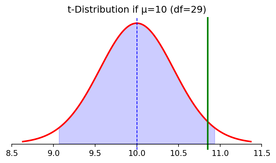
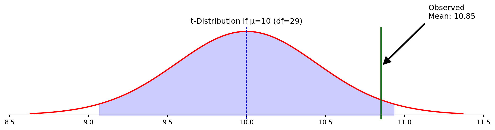
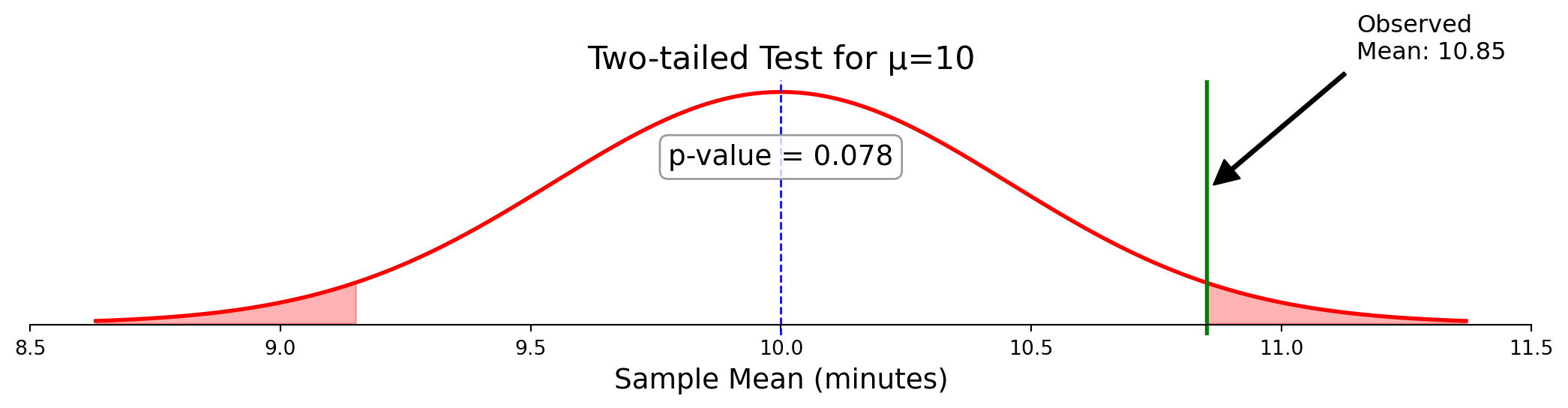
✅ Correct: The probability of observing a test statistic at least as extreme as ours, if \(H_0\) were true

• It measures the compatibility between our data and the null hypothesis.
• Example: A p-value of 0.04 means: “If the null hypothesis were true, we’d see results this extreme or more extreme only about 4% of the time.”

> think of it like this: The p-value answers “How surprising is this data if the null hypothesis is true?” not “Is the null hypothesis true?”

Looking Forward: Bivariate GLM

This framework extends directly to regression analysis.

Next time:

• Bivariate GLM: Comparing means between two groups

> the hypothesis testing framework is foundational for modern science

Looking Forward: Regression

This framework extends directly to regression analysis.

Today’s model: \(E[y] = \beta_0\) (just an intercept)

Next: \(E[y] = \beta_0 + \beta_1 x\) (intercept and slope)

• Each \(\beta\) coefficient will have its own t-test
• Same framework: estimate ± t-critical × SE
• The t-distribution accounts for uncertainty in our estimates

> regression is just an extension of what we learned today

Summary

We’ve built the foundation for statistical modeling.

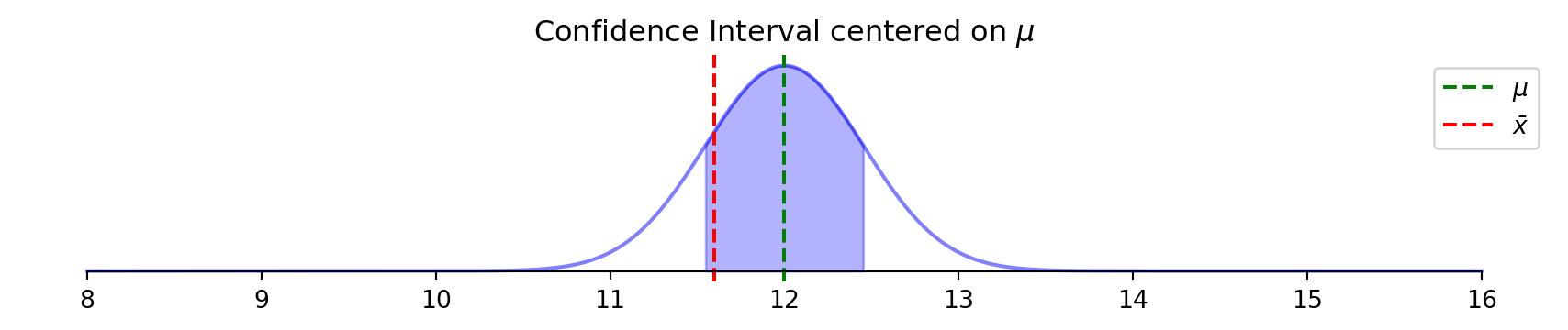
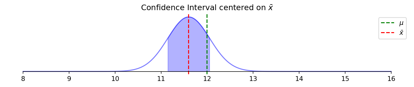
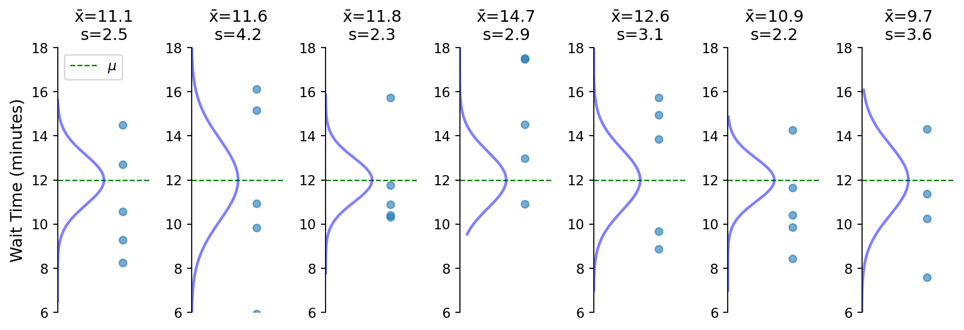
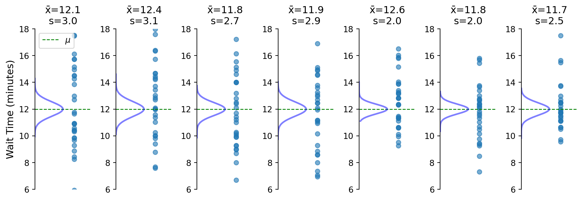
• Flipped perspective: center on what we observe (\(\bar{x}\)) not what’s unknown (\(\mu\))
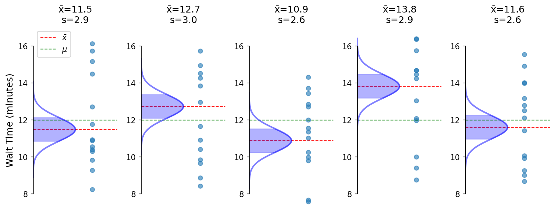
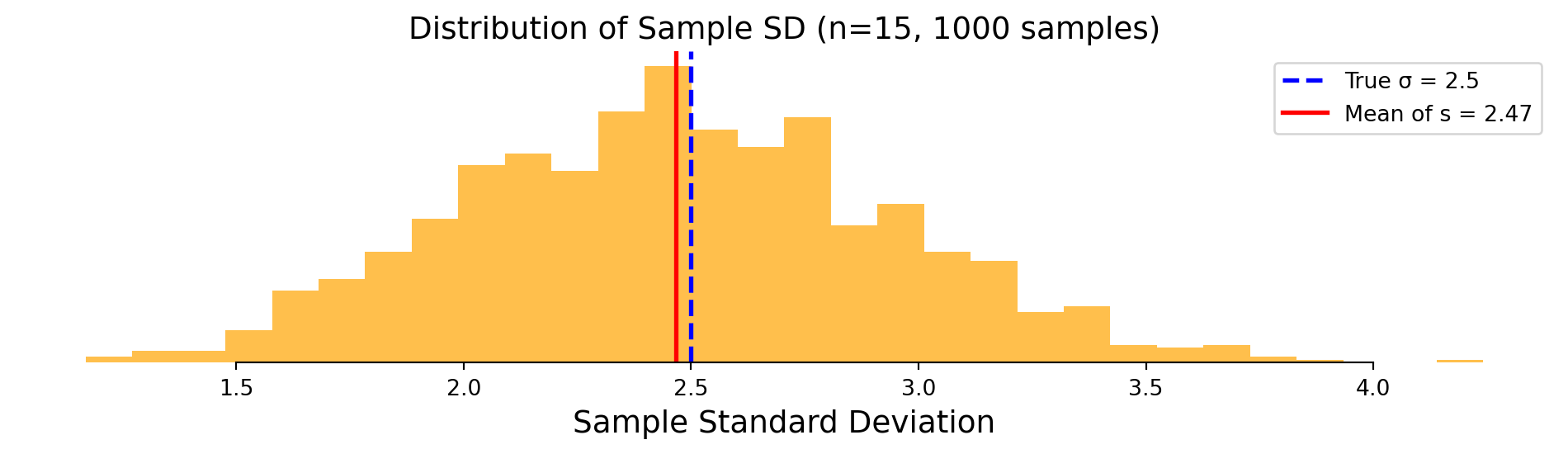
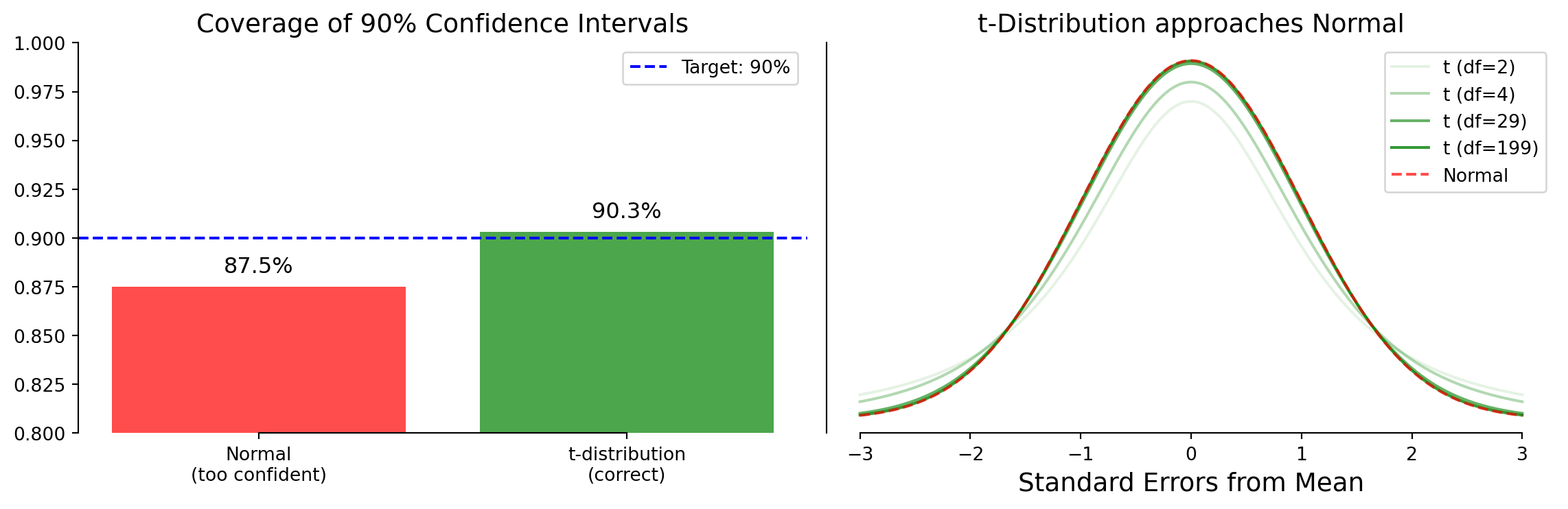
• Sample SD varies, creating need for t-distribution
• Built our first model: \(E[y] = \beta_0\)
• Tested hypotheses by shifting data
• Connected hypothesis tests to confidence intervals

> these tools form the foundation of econometric analysis