ECON 0150 | Economic Data Analysis

The economist’s data analysis skillset.

Dr. Taylor Weidman

taylorjweidman@pitt.edu | 4702 Posvar Hall

ECON 0150 | Economic Data Analysis

How economists do data analysis.

Dr. Taylor Weidman

taylorjweidman@pitt.edu | 4702 Posvar Hall

ECON 0150 | Economic Data Analysis

How economists do data analysis.

Taylor

taylorjweidman@pitt.edu | 4702 Posvar Hall

ECON 0150 | Economic Dada Analysis

How economists do data analysis.

Taylor

taylorjweidman@pitt.edu | 4702 Posvar Hall

ECON 0150 | Economic Dada Analysis

How economists do data analysis.

What is economic dada analysis?

The data analysis done by economist fathers :)

What is economic data analysis?

The data analysis done by economists :)

Economists use data to build models and inform decisions.

Describing the landscape of economics

• Have incomes risen in the last year?
• How has unemployment changed?
• Has the racial wealth gap narrowed?

Distinguishing between economic theories

• Do voters with neighbors of the same party vote more?
• Does the gender of a Lyft driver impact rates of tipping?
• Is cooperation higher in ‘easier’ repeated prisoner’s dilemmas?

Course Goals

Developing the data analysis pipeline used by economists.

Skillset 1. Summarize data (tables and figures).
Skillset 2: Build and interpret models (general linear model).
Skillset 3: Communicate findings (writting and presentations).

Goal: I want you to be able to build appropriate statistical models for new problems and interpret their results.

Course Structure

The course is divided into six parts.

Part 1: Exploring Variables
Part 2: Exploring Relationships
Part 3: Univariate General Linear Model
Part 4: Bivariate General Linear Model
Part 5: Multivariate General Linear Model
Part 6: Communicating with Data

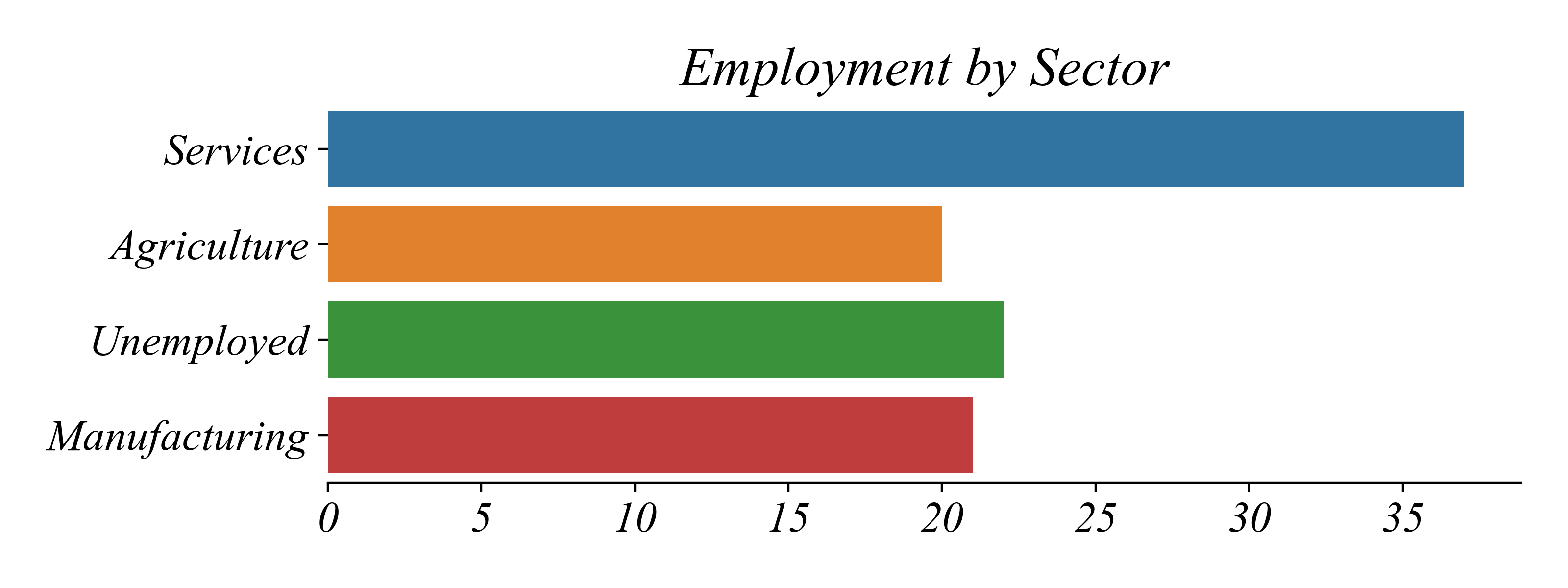
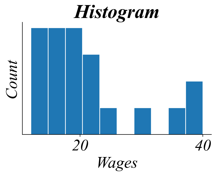
Part 1: Exploring Variables

Focus: Understanding single variables through summarization (eg. tables and figures).

Example: Analyzing a dataset of wages.

Wage	EduYrs
12	8
13	10
14	10
14	11
15	12

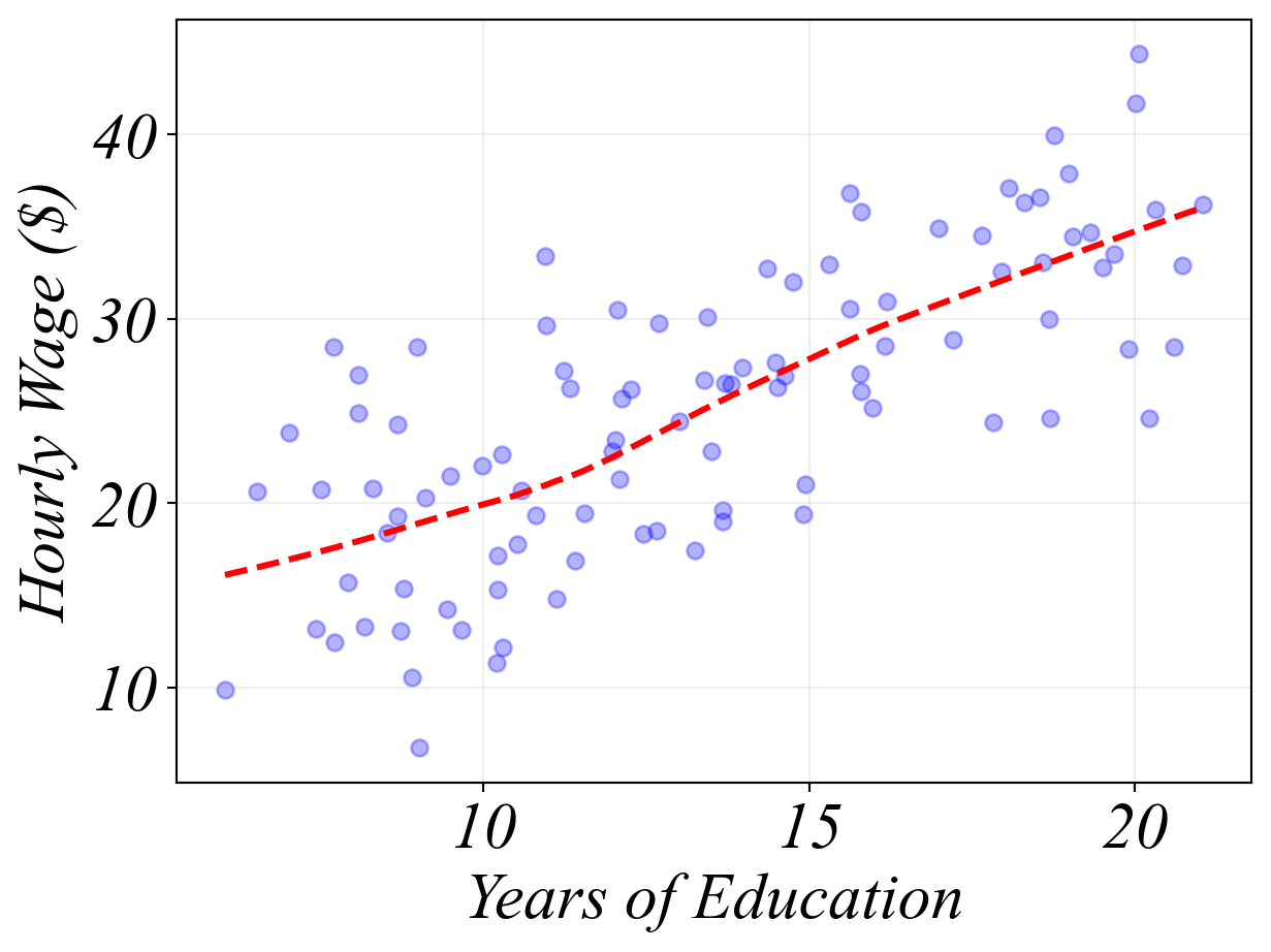
Part 2: Exploring Relationships EDA

Focus: Understanding relationships between variables (eg. scatterplot).

Example: Exploring a relationship - education and wages.

	Wage	EduYrs
0	14	10
1	15	12
2	16	12
3	18	13
4	18	14
5	20	14
6	22	15

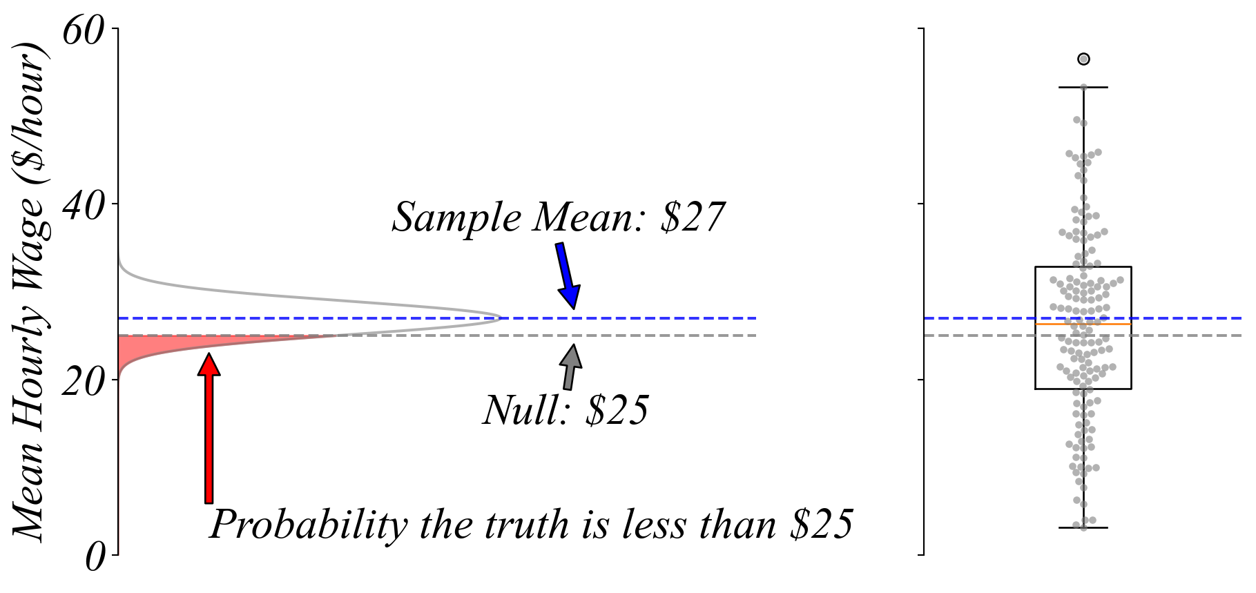
Part 3: Univariate General Linear Model

Focus: Sampling variation, Central Limit Theorem, and basic testing.

Example: Is the difference from $25 a real pattern or just noise?

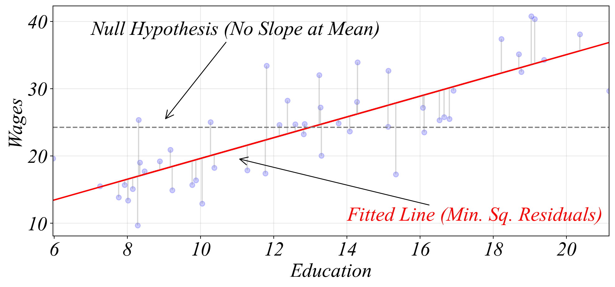
Part 4: Bivariate General Linear Model

Focus: Regression and residual analysis.

Example: Is the positive slope a real pattern or just noise?

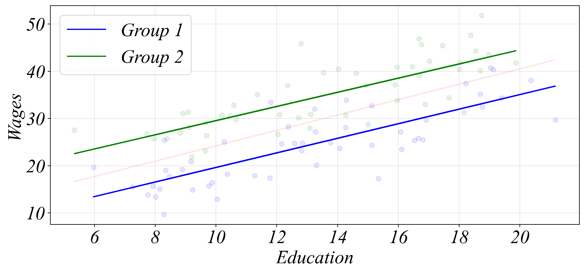
Part 5: Multivariate General Linear Model

Focus: Fixed effects, control variables, interactions.

Example: Do different groups have different relationships?

Part 6: Communicating with Data

Focus: Clear narratives, effective visualization, presentation skills.

Examples: Some student work from last semester!

Course Logistics

Resources & Tools

Software: Excel & Python

Website: ECON_0150

Optional Textbooks:

• Data Visualization and Analysis in R by Dustin Fife
• How Charts Lie by Alberto Cairo
• Analysis of Economic Data (2nd ed.) by Gary Koop

Your Work

Exercises (10%)

• Together in class; lowest 3 dropped.

Homework (10%)

• Fridays by 5PM; lowest 3 dropped.
• No-questions-asked extensions through Sunday at Midnight.

MiniExams (1 × 20% + 1 × 15% + 1 × 10% + 1 × 5% + 1 × 0% = 50%)

• Roughly every two weeks; beginning of class
• Open-book, open-note (no electronics).

Your Work

Final Project (30%)

• One small project per part.
• Presentation + paper at the end of the semester.
• Demonstrate full analysis from start to finish.

Attenance (1% extra)

• Just a small gift

Policies

Email Policy:

• Response may take up to 1-2 days.
• Be concise with your questions.
• My email is off evenings and weekends.

AI Policy:

• Encouraged as a learning and coding tool :)
• Your work must be your own.
• Cite your source.

Academic Conduct: Adhere to the Academic Integrity Code.

Looking Ahead

First Homework:

• Due (next) Friday Jan 23rd at 5PM on Gradescope

First MiniExam:

• First class of Week 4 (Feb 3) during the first 20 minutes.
• Bonus “preview” question on material not yet covered.

Getting Set Up

Excel:

• Free for students through Pitt’s institutional access

Python:

• Google Colab Notebooks (recommended)

Survey Fall 2025

Where are students coming from?

Lets measure hometown using distance

Where are students coming from?

Lets measure hometown using distance

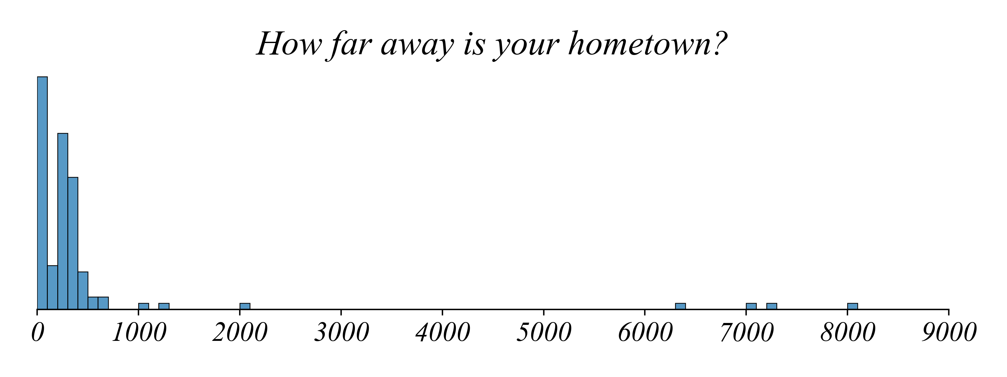
> quite a few people come internationally :)

> lets zoom in a bit to see more details about closer distances

Where are students coming from?

Lets measure students hometown using distance

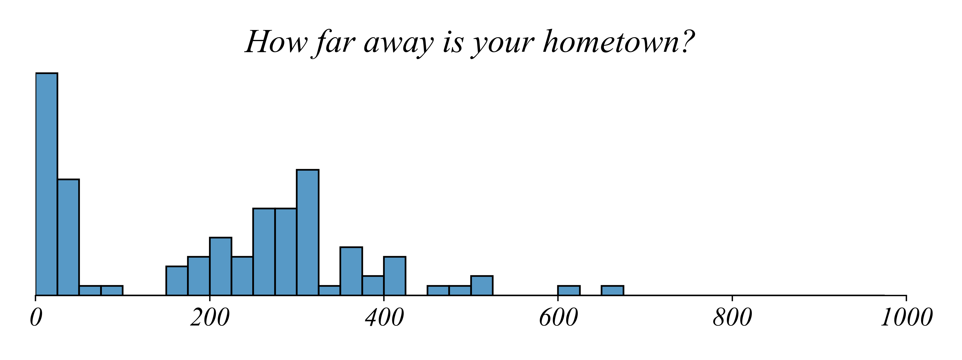
> many from Pittsburgh and the Philly area

When were students born?

Lets use birthyear

When were students born?

Lets use birthyear

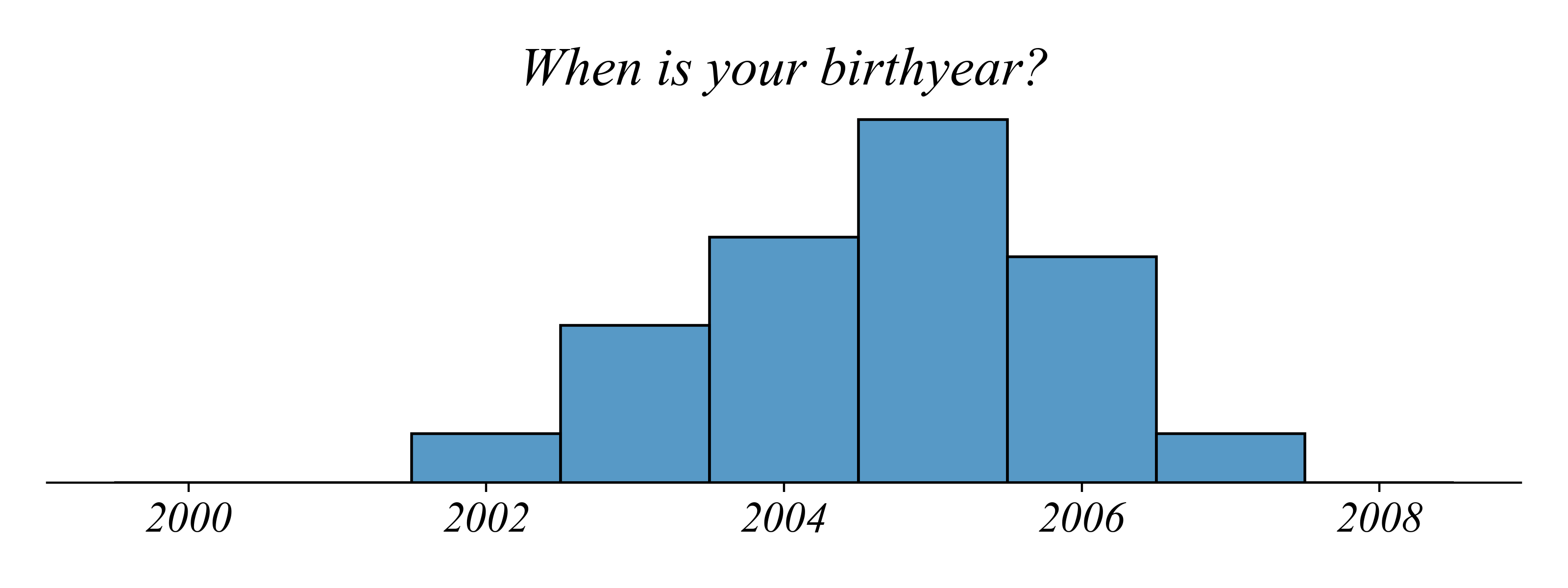
> the most common birthyear was 2005

What are students majors?

Sorry if you’re not on the list or have multiple :)

What are students majors?

Sorry if you’re not on the list or have multiple :)

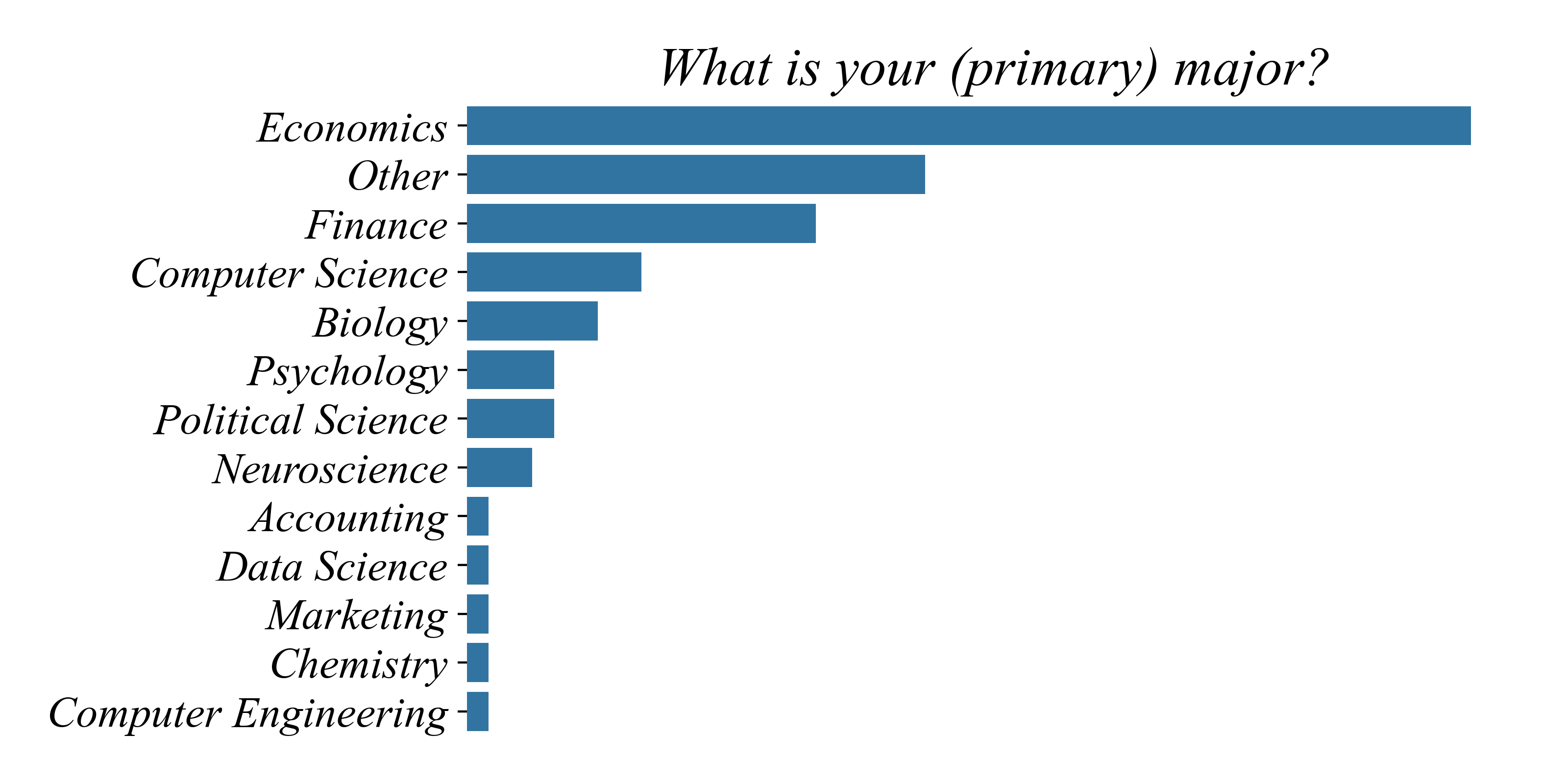
> most are Econ and many not on my limited list

Did you like your stats class?

It’s a prereq for the class

Did you like your stats class?

It’s a prereq for the class

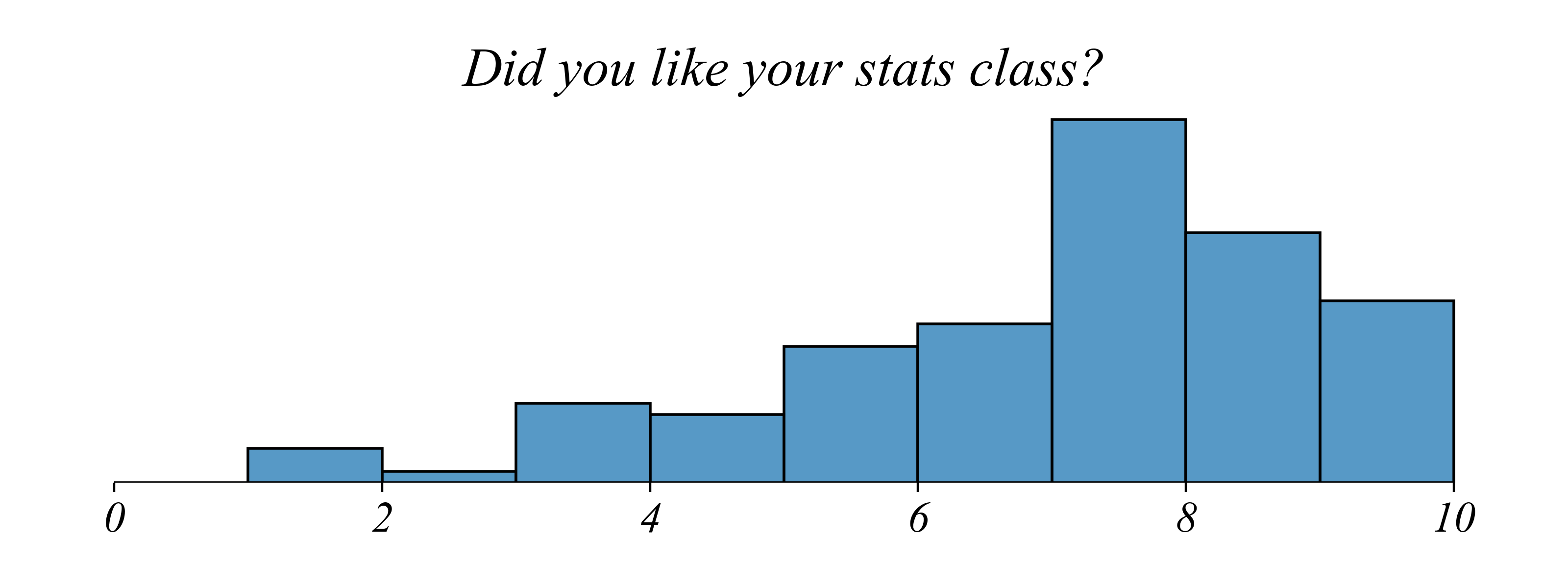
> most generally liked it; some did not

Is stats related to your excitement for this class?

I would suspect a positive relationship

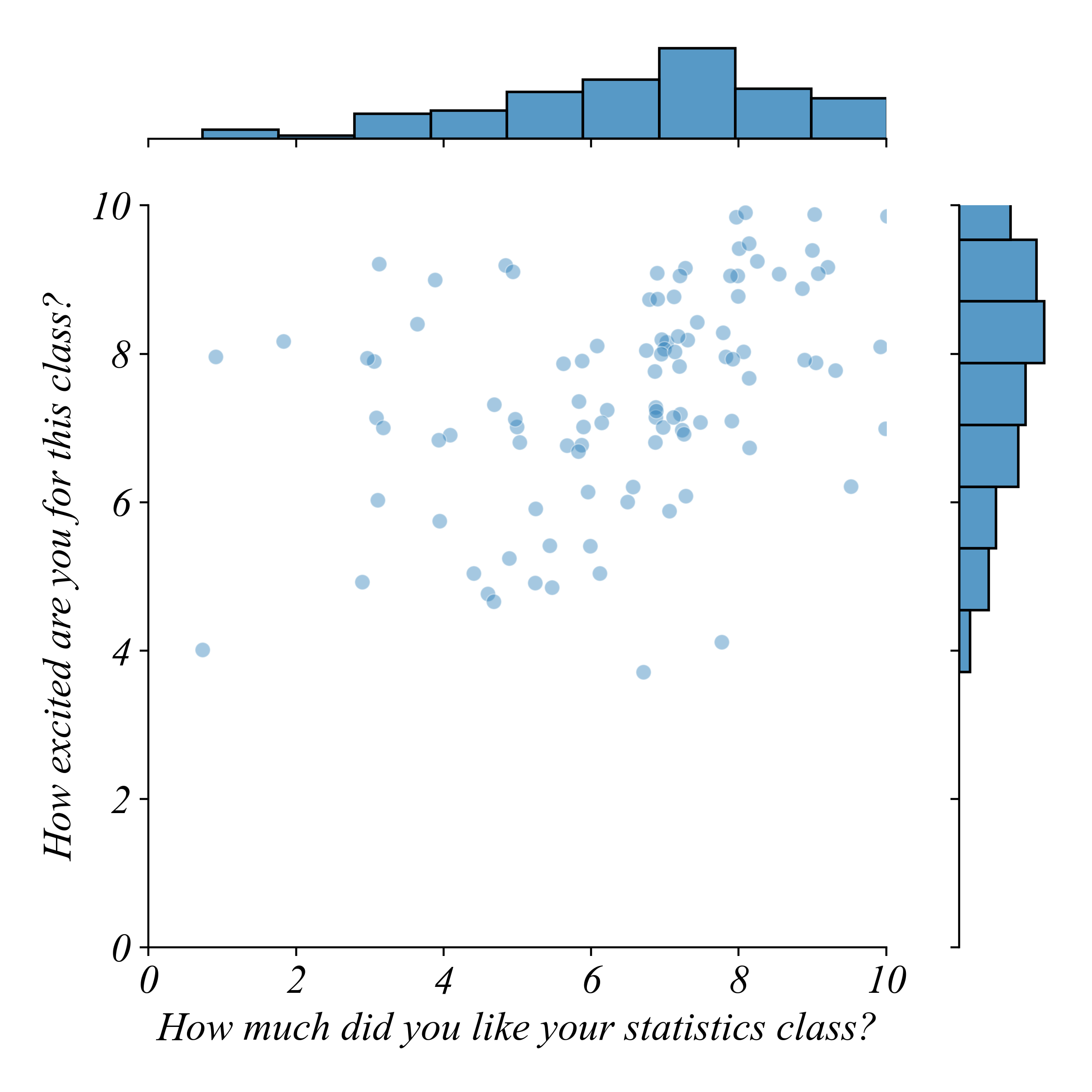
Is stats related to your excitement for this class?

I would suspect a positive relationship

Is confidence in Excel related to class excitement?

I would expect it is

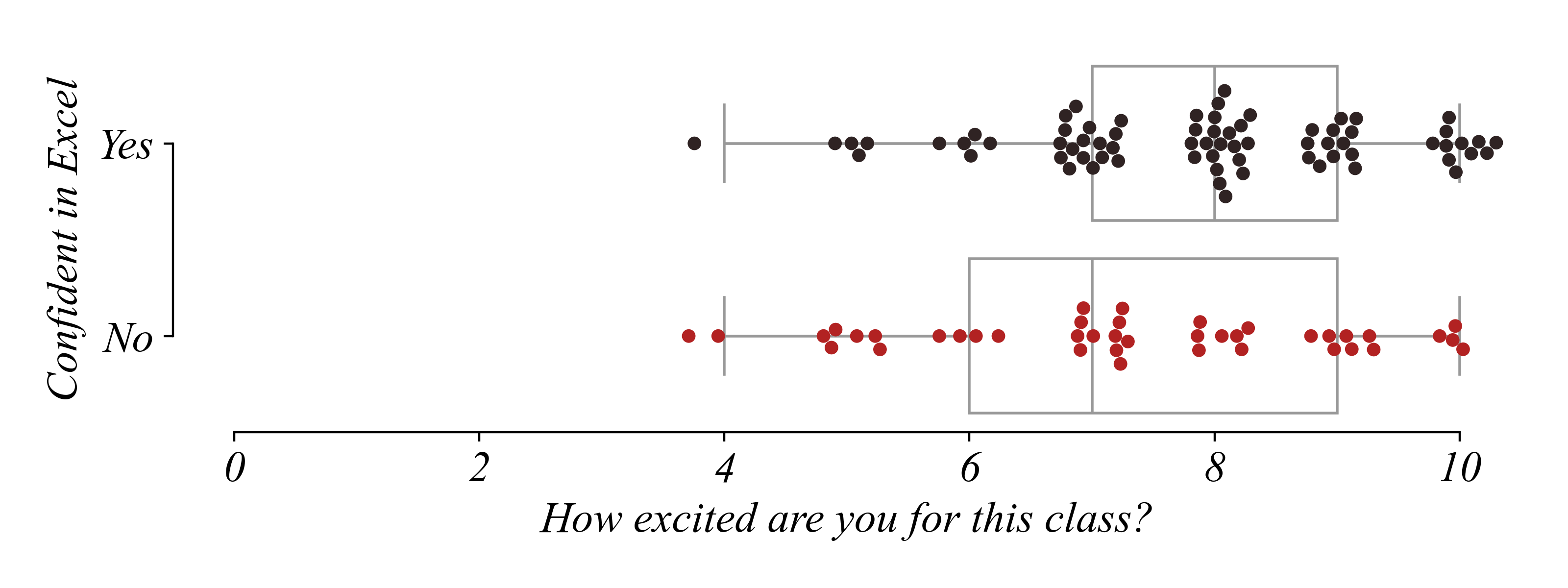
Is confidence in Excel related to class excitement?

I would expect it is

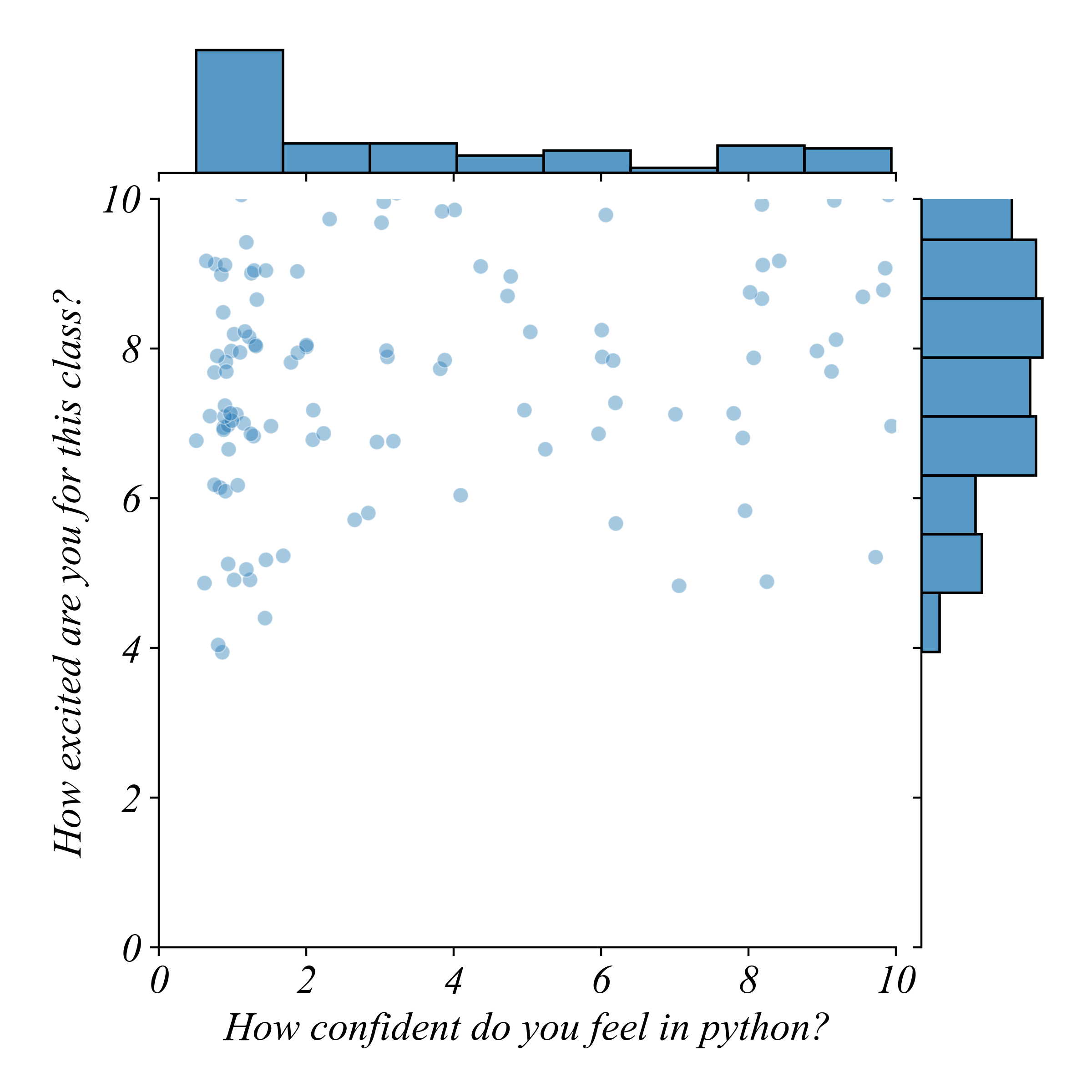
Is confidence in python related to excitement?

Again I would expect it is

ECON 0150 | Economic Data Analysis

Why does economic data analysis matter?

A case study in minimum wage policy

Dr. Taylor Weidman

taylorjweidman@pitt.edu | 4702 Posvar Hall

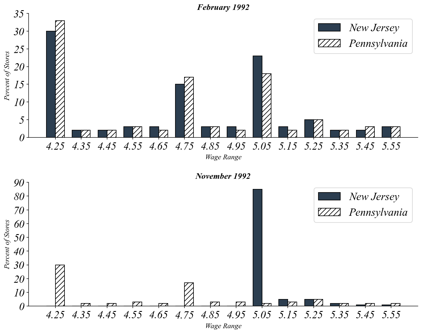
New Jersey, 1992

A state raises its minimum wage.

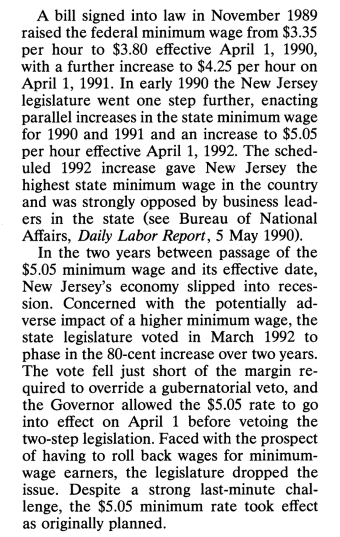
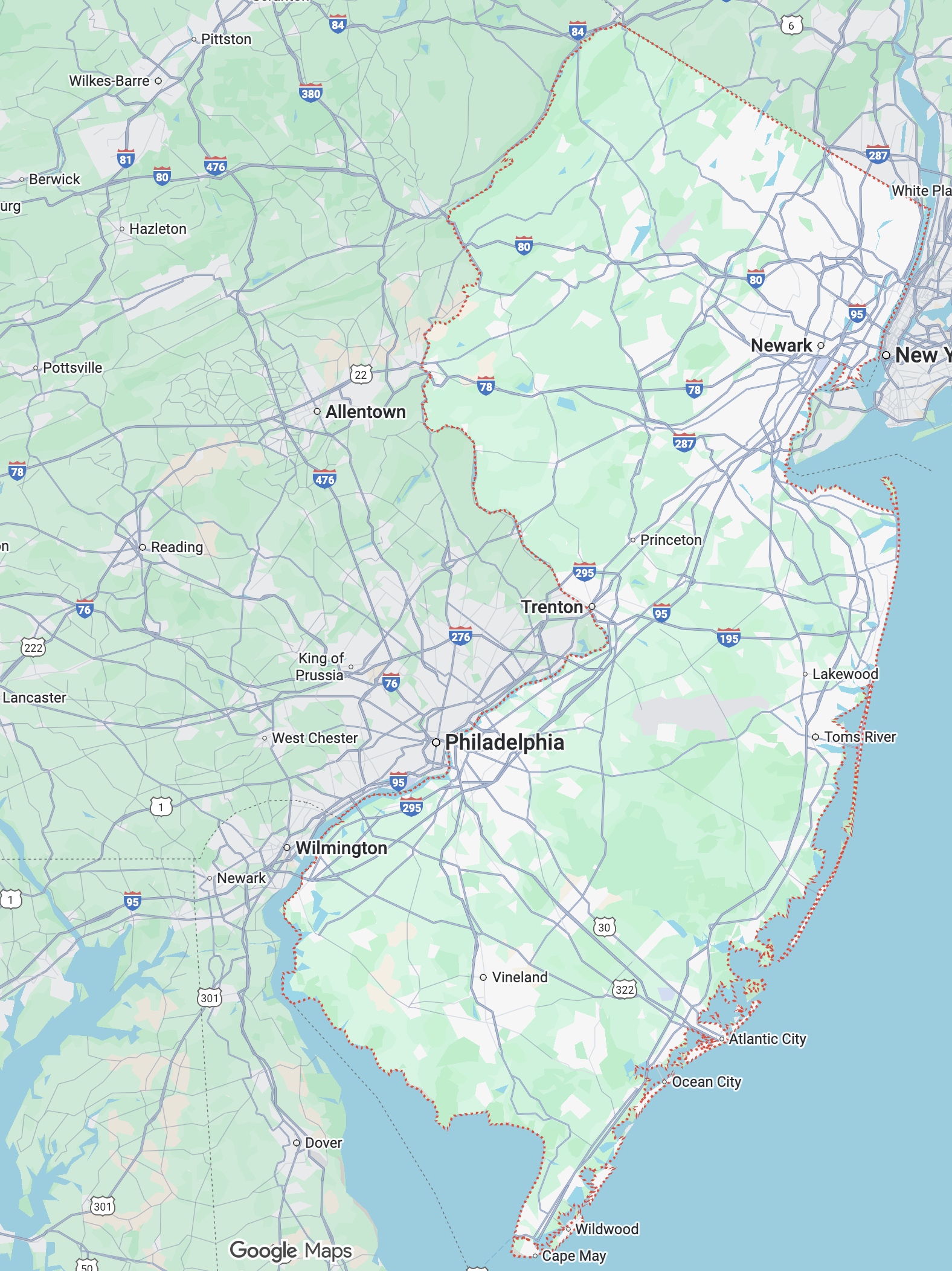
New Jersey, 1992

A natural experiment.

	NJ	PA
March 1992	$4.25	$4.25
April 1, 1992	$5.05	$4.25

What happens to employment?

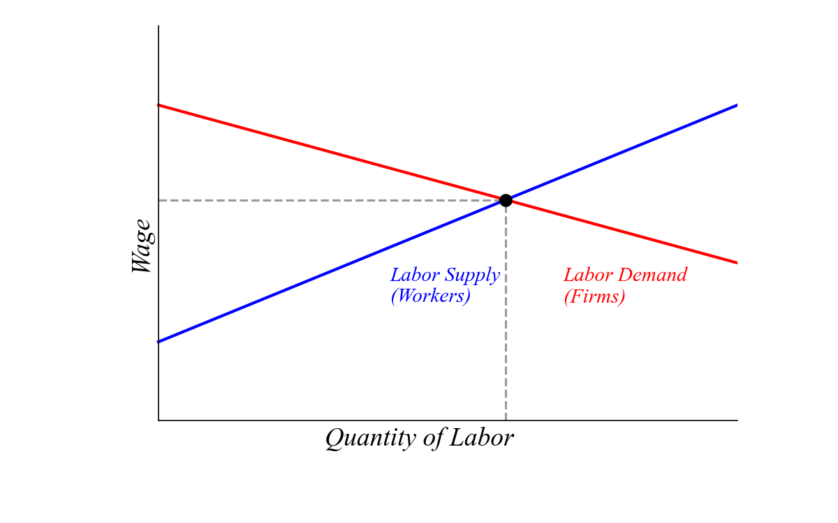
Economic Theory

Supply and demand.

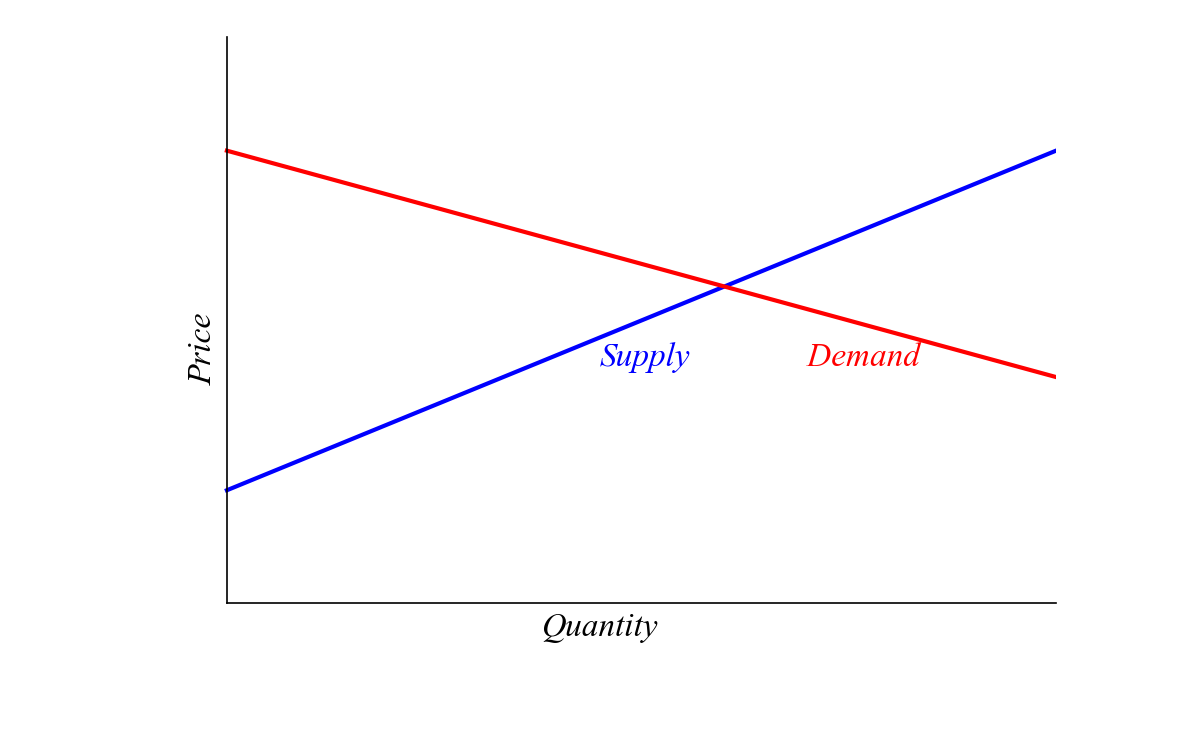
Economic Theory

Equilibrium.

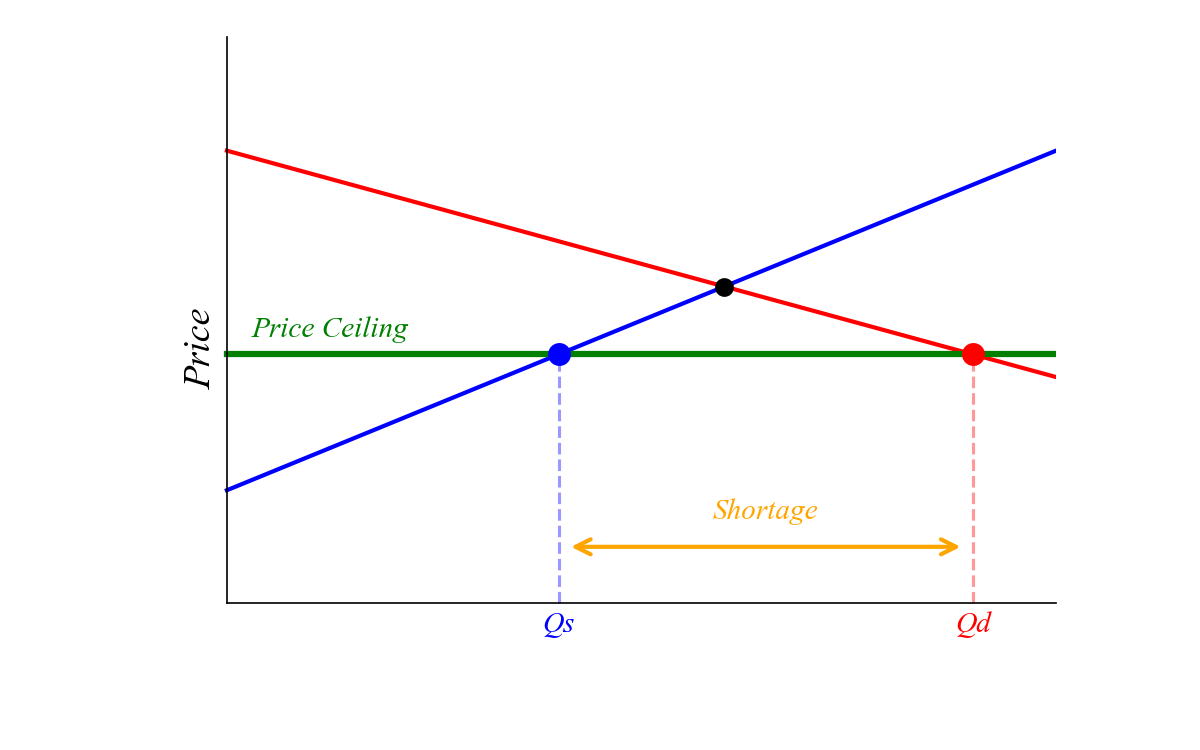
Economic Theory

A binding price ceiling creates a shortage.

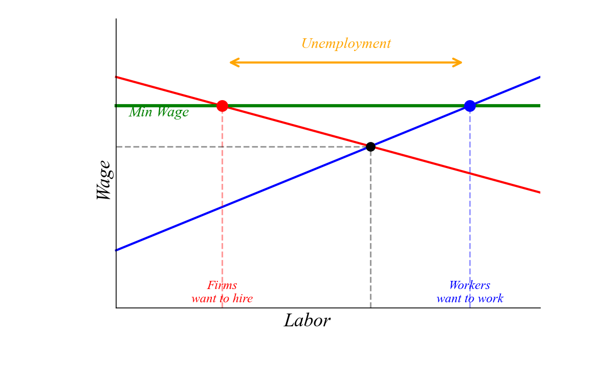
Economic Theory

A binding price floor creates a surplus.

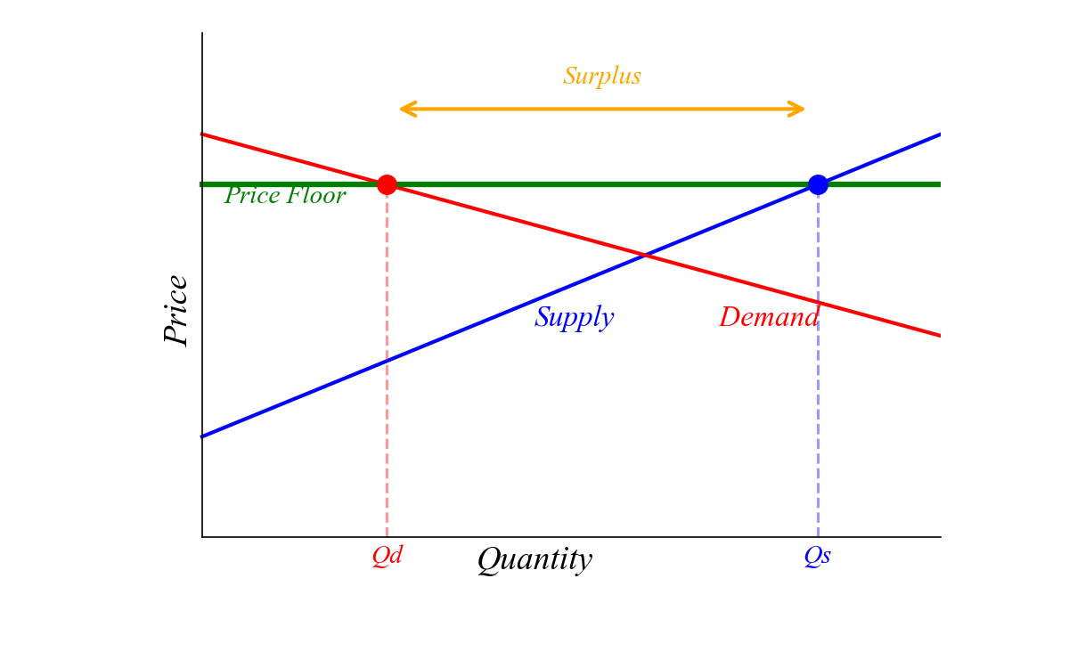
Economic Theory

The labor market.

Economic Theory

A minimum wage is a price floor in the labor market.

Card and Krueger

Two economists decided to find out.

David Card

Alan Krueger

Data

Surveying fast-food restaurants before and after.

	Wave 1	Wave 2
Timing	Feb-Mar 1992	Nov-Dec 1992
Policy	Before increase	After increase
Stores	410	399

Burger King, KFC, Wendy’s, Roy Rogers in NJ and eastern PA

Data

Before the minimum wage increase.

	New Jersey	Pennsylvania
Stores surveyed	331	79
FTE employment	20.4	23.3
Starting wage	$4.61	$4.63
Wage = $4.25	30.5%	32.9%

Data

Wages shifted to the new minimum.

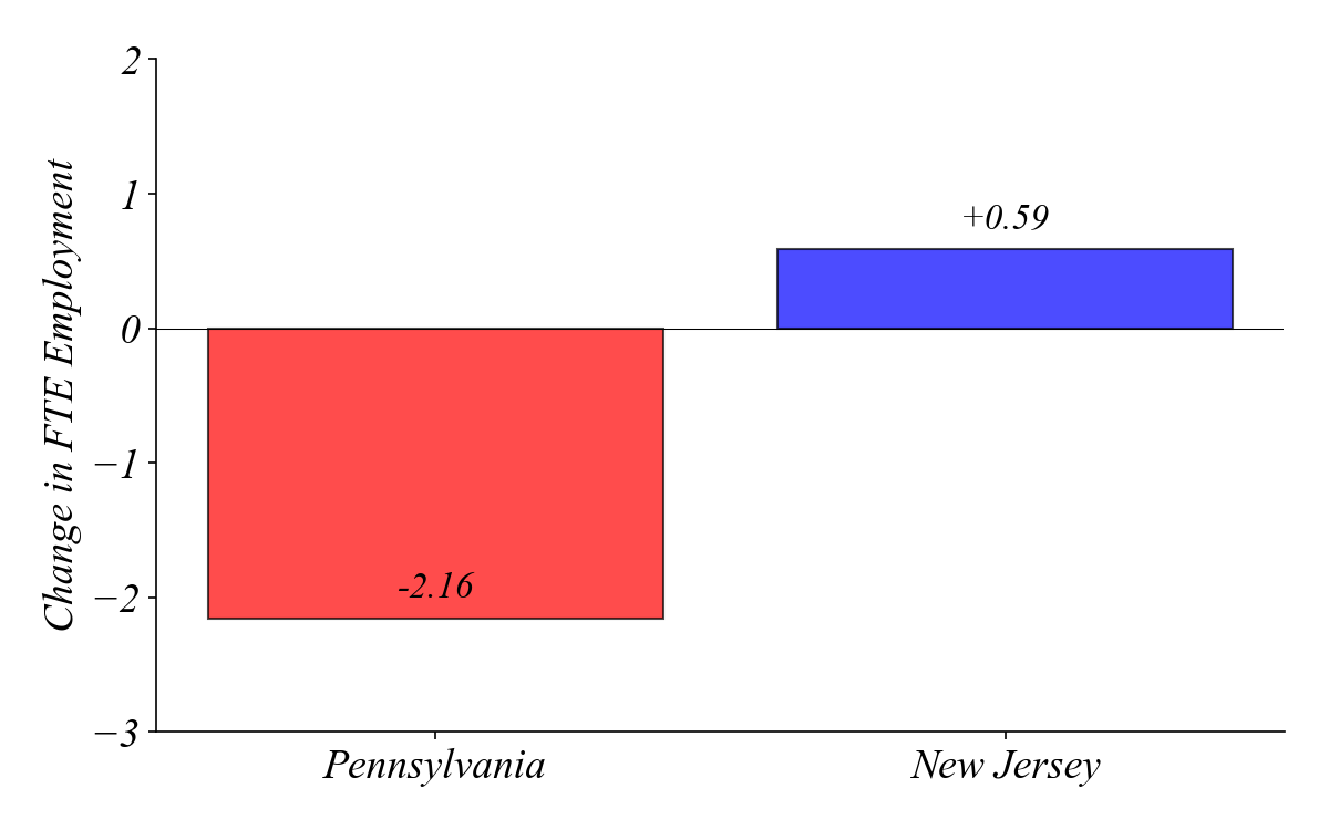
Analysis

Difference-in-differences.

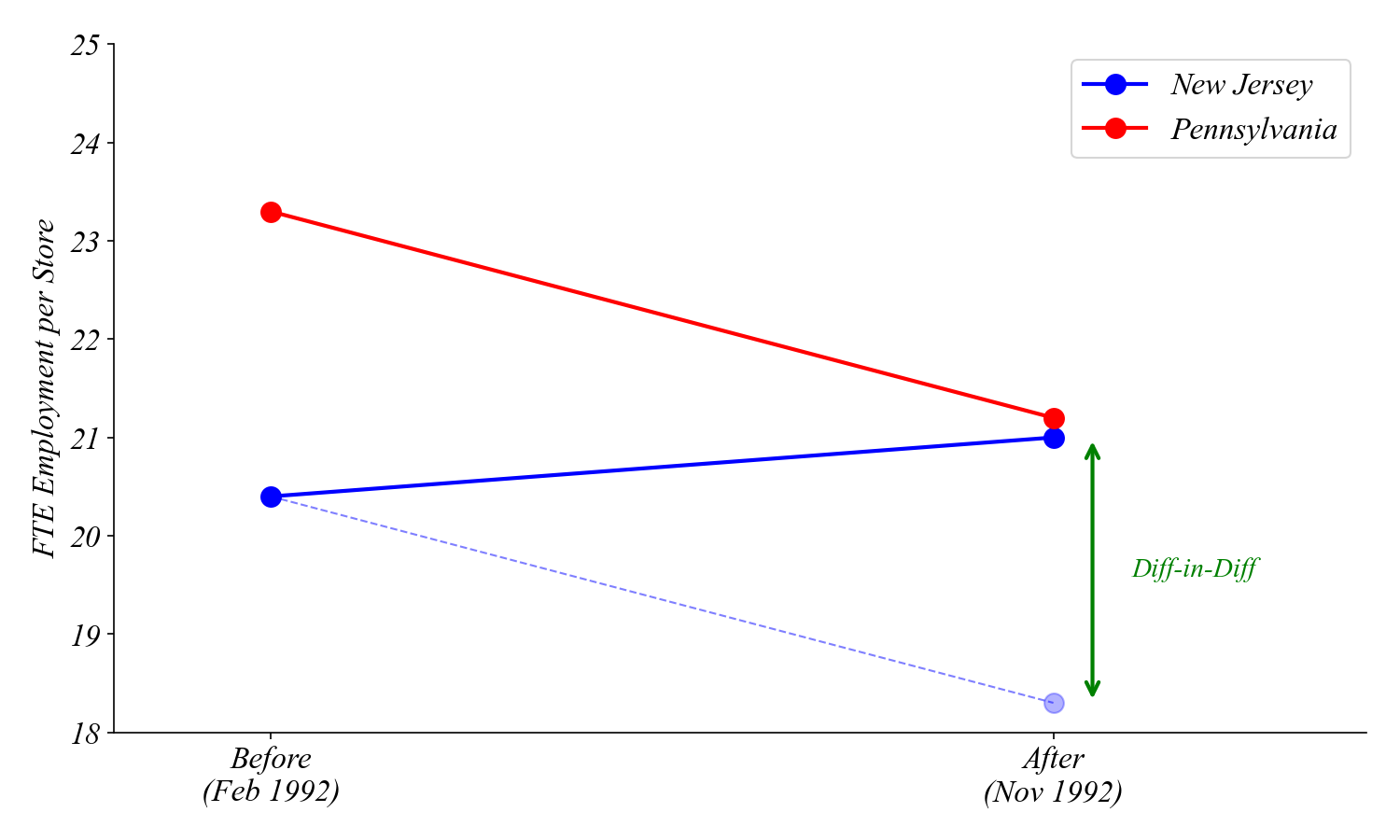
Results

Employment did not fall in New Jersey.

FTE Employment	Pennsylvania	New Jersey	Difference
Before	23.33	20.44	-2.89
After	21.17	21.03	-0.14
Change	-2.16	+0.59	+2.76

Results

Employment did not fall in New Jersey.

Theory vs. Evidence

The data told a different story.

Theory prediction

• higher minimum wage → lower employment

Data showed

• no decrease in employment

“Contrary to the central prediction of the textbook model… we find no evidence that the rise in New Jersey’s minimum wage reduced employment.”

— Card and Krueger (1994)

Let’s learn how to do this kind of analysis.

What is Data?

Data is a sample drawn from a process we want to understand.

\[x \sim F\]

• \(x\) = what we observe (our data)
• \(F\) = what generated it (the random variable)

We have \(x\). We care about \(F\).

Two skills:

1. Description (Parts 1 - 2) — Summarize \(x\).
2. Inference (Parts 3 - 5)— Learn about \(F\) from \(x\).

How Do We Organize Data?

Notation helps keep things organized.

We write \(x_{it}\) where:

• i (unordered) indexes entities (eg. people, firms, countries)
• t (ordered) indexes time (eg. days, months, years)

This distinguishes substantive variables (what we measure) from index variables (how we organize).

Dimensions of Data

Data structure; variable type; number of variables.

Data Structure (\(i\),\(t\))

• Cross-sectional
• Timeseries
• Panel

Variable Type (\(x\))

• Categorical
• Numerical

Number of Variables (\(n\))

• Univariate (n=1)
• Bivariate (n=2)
• Multivariate (n>2)

Data Structures

Which indices (\(i\), \(t\)) are active?

	What varies	Example
Cross-section	Entity (i)	Household incomes in 2024
Time series	Time (t)	Average US income from 1950–2024
Panel	Both (i and t)	Income across households, 1950–2024

Variable Types

What are the values (\(x\))?

		Definition	Example
Categorical	Binary	Two categories	Employed (YES/NO)
	Nominal	Unordered	Blood type (A, B, AB, O)
	Ordinal	Ordered	Education (HS, BA, MA, PhD)
Numerical	Discrete	Countable	Number of children
	Continuous	Real numbers	Household income

How We Work with Data

Three steps, every time.

1. SELECT — What does our data contain?

2. TRANSFORM — How do we change the data to make it more useful?

3. ENCODE — How do we turn values into visual elements?

Course Progression

Building complexity along two axes.

Part	Focus	Key question
0	Framework	What tools do we need?
1	Variables	What does this variable look like?
2	Relationships	How do these variables relate?
3	Univariate GLM	What can we infer about the population?
4	Bivariate GLM	How does y change with x?
5	Multivariate GLM	How does y change with x, controlling for z?

How Each Class Works

A consistent rhythm.

When	What	Purpose
Before class	Concept video	Learn core ideas at your pace
Start of class	Quiz	Confirm your understanding
During class	Exercise	Guided practice with support
After class	Homework	Independent practice

Exercises are homework prep.

Let’s begin.

Exercise 0 | Diagram Data

Q1. Identify the data structure, variable type, indices, and number of variables for dataset1.csv.

Year	Real_GDP
1970	5.316
1971	5.491
1972	5.780
1973	6.106
…	…

Index: \(t\) (Year)

Structure: Time series

Variable: Continuous

N Variables: Univariate

Exercise 0 | Diagram Data

Q1. Visualize dataset1.csv.

Exercise 0 | Diagram Data

Q2. Identify the data structure, variable type, indices, and number of variables for dataset2.csv.

Household ID	Employment Status
D001	Unemployed
D002	Employed
D003	Employed
D004	Employed
…	…

Index: \(i\) (Household)

Structure: Cross-sectional

Variable: Binary

N Variables: Univariate

Exercise 0 | Diagram Data

Q2. Visualize dataset2.csv.

Exercise 0 | Diagram Data

Q3. Identify the data structure, variable type, indices, and number of variables for dataset3.csv.

Household ID	Year	Income	Savings
H001	2010	34,610	6,157
H001	2011	45,560	2,506
H001	2012	83,698	8,789
H002	2010	52,341	4,123
…	…	…	…

Index: \(i\) (Household), \(t\) (Year)

Structure: Panel

Variable: Continuous

N Variables: Bivariate

Exercise 0 | Diagram Data

Q3. Visualize dataset3.csv.

Exercise 0 | Diagram Data

Q4. Identify the data structure, variable type, indices, and number of variables for dataset4.csv.

ID	Economic Optimism
B001	Somewhat Pessimistic
B002	Very Pessimistic
B003	Somewhat Optimistic
B004	Very Optimistic
…	…

Index: \(i\) (Person)

Structure: Cross-sectional

Variable: Ordinal

N Variables: Univariate

Exercise 0 | Diagram Data

Q4. Visualize dataset4.csv.

Exercise 0 | Diagram Data

Q5. Identify the data structure, variable type, indices, and number of variables for dataset5.csv.

ID	Sector
A001	Services
A002	Agriculture
A003	Unemployed
A004	Manufacturing
…	…

Index: \(i\) (Person)

Structure: Cross-sectional

Variable: Nominal

N Variables: Univariate

Exercise 0 | Diagram Data

Q5. Visualize dataset5.csv.